Today it occurred to me that I have not updated my blog for a long time; lately I have been busy with written tests and interviews, and with my graduation project. Now that things have come to a pause today, I might as well organize the Xgboost model I reviewed a few days ago and post an article.
Tree ensemble
Ensemble algorithms are a broad and very important class of algorithms in machine learning, generally divided into Bagging and Boosting. Ensembling decision trees is of course a customary technique. For tree ensembles, the representative of the Bagging method is Random Forest, which randomly groups attributes and data for decision tree learning and finally aggregates the results; the representative of the Boosting method is AdaBoost and GBDT (gradient boosted decision trees). These algorithms are all quite important and cannot be summed up in a sentence or two, so I will not expand on them. Within tree Boosting, Tianqi Chen proposed a new model, Xgboost. This model makes use of the second derivative of the objective function and also adds a regularization term to prevent the model from overfitting. Below is an interpretation of the Xgboost model.
Objective function
The result of a tree ensemble model is generated from the results of many individual tree models. The individual tree model chosen by Xgboost is CART. The CART model differs somewhat from other decision tree models: the value of its leaves is a definite score rather than an actual class, which helps to implement highly efficient optimization algorithms. Using a bunch of CART trees for prediction, we can simply add up the results of the individual CART models. This gives the following function:
$$ \hat{y}_i = \Phi(\mathbf{x}_i) = \sum_{k=1}^K f_k(\mathbf{x}_i), \ f_k \in F \tag{1} $$where the given dataset has n rows of data and m features. $D=\{(\mathbf{x}_i,y_i)\}(\vert{D}\vert=n,\mathbf{x}_i\in R^m,y_i\in R)$ and an additive algorithm is used.
$F=\{f(\mathbf{x})=w_{q(\mathbf{x})}\}(q:R^m\rightarrow T.\ w\in R^T)$ is the space of all possible CART trees, and $f(x)$ is a single CART tree model. $T$ is the number of leaf nodes of the tree, $q(x)$ maps a sample to some value from 1 to T, that is, to some leaf node; in fact it represents the structure of the tree, and $w_{q(x)}$ is the prediction of this tree for the sample.
The objective function to be optimized can then be defined as:
$$ L(\Phi) = \sum_i l(\hat{y}_i, y_i)+\sum_k \Omega(f_k) \tag{2} $$where $L(\hat{y}_i,y_i)$ is the loss function and the latter term is the regularization term representing the complexity of the tree:
$$ \Omega(f) = \gamma T+\frac{1}{2}\lambda{\Vert{w}\Vert}^2 \tag{3} $$Usually the mean squared error (MSE) is chosen as the loss function, which gives a very pretty form:
$$ L^{(t)} = \sum_{i=1}^n [2(\hat{y}^{(t-1)}_i-y_i)f_t(x_i)+{f_t(x_i)}^2]+\Omega(f_t)+const $$For other loss functions (as long as their second derivative exists), Taylor’s formula is used to expand $L^{(t)}(y_i,\hat{y}^{(t-1)}_i+f_t(x_i))$ to the second order, where we let $x=\hat{y}_i^{(t-1)}+f_t(x_i), \ x_0=\hat{y}_i^{(t-1)}$:
$$ \begin{aligned} L^{(t)}(y_i,x) & \simeq l(y_i,x_0)+l^\prime(y_i,x_0)\cdot(x-x_0)+\frac{1}{2!}l^{\prime\prime}(y_i,x_0)\cdot{(x-x_0)}^2+\Omega(f)+const \\ & = l(y_i,x_0)+\frac{\partial l(y_i,x_0)}{\partial x_0}f_t(x_i)+\frac{1}{2}\frac{\partial^2 l(y_i,x_0)}{\partial^2 x_0}f_t^2(x_i)+\Omega(f)+const \end{aligned} \tag{4} $$Let $g_i = \frac{\partial l(y_i,x_0)}{\partial x_0}$, $h_i = \frac{\partial^2 l(h_i, x_0)}{\partial^2 x_0}$, and ignore the constant term, giving:
$$ \tilde{L}^{(t)} = \sum_{i=1}^n[g_if_t(x_i)+\frac{1}{2}h_if_i^2(x_i)]+\Omega(f_t) \tag{5} $$Define $I_j=\\{i\vert q(\mathbf{x}_i)=j\\}$ as the set of indices of the training samples assigned to leaf j. Combining equations (3) and (5) gives:
$$ \begin{aligned} \tilde{L}^{(t)} & = \sum_{i=1}^n[g_if_t(x_i)+\frac{1}{2}h_if_i^2(x_i)]+\gamma T+\frac{1}{2}\lambda \sum_{j=1}^T{w_j}^2 \\ & = \sum_{j=1}^T[(\sum_{i \in I_j}g_i)w_i+\frac{1}{2}(\sum_{i \in I_j}h_i+\lambda){w_j}^2]+\gamma T \end{aligned} \tag{6} $$For a determined tree structure $q(x)$, the optimal weight $w$ of leaf node j can be computed as follows:
$$ w_j^* = -\frac{\sum_{i \in I_j}g_i}{\sum_{i \in I_j}h_i+\lambda} \tag{7} $$and the corresponding loss is:
$$ \tilde{L}^{(t)}(q) = -\frac{1}{2}\sum_{j=1}^{T}\frac{(\sum_{i \in I_j}g_i)^2}{\sum_{i \in I_j}h_i+\lambda}+\gamma T \tag{8} $$Equation (8) can be used to evaluate how good a tree model is; the smaller the value the better. This value is only used to measure the quality of the tree structure and has nothing to do with the values of the leaf nodes. This can be seen from the derivation: $\tilde{L}^{(t)}(q)$ depends only on $g_i$ and $h_i$, and these two values depend only on the structure of the tree, having nothing to do with the leaf node values.
Growing the tree
Obviously a CART tree has infinitely many structures, so growing a tree and then evaluating the structure is not realistic. There is a greedy algorithm that grows the tree layer by layer. That is, starting from the root node, branches are created layer by layer. Suppose $I_L$ and $I_R$ are the instances contained in the left and right nodes after branching, with $I = I_L \bigcup I_R$; then the criterion for whether to branch is:
$$ L_{split} = \frac{1}{2}\left[\frac{(\sum_{i \in I_L}g_i)^2}{\sum_{i \in I_L}h_i+\lambda}+\frac{(\sum_{i \in I_R}g_i)^2}{\sum_{i \in I_R}h_i+\lambda}-\frac{(\sum_{i \in I}g_i)^2}{\sum_{i \in I}h_i+\lambda}\right]-\gamma \tag{9} $$The positive and larger the value of $L_{split}$, the more worthwhile the branch is, because after branching $\tilde{L}^{(t)}(q)$ becomes smaller. In fact, $\gamma$ acts as a threshold; the larger this value, the stricter the branching criterion.
Note: Xgboost does not need a separate pruning operation, because the complexity of the tree model is already taken into account when growing the tree, which corresponds to the parameter $\gamma$.
The algorithm model for finding the best split point based on the greedy algorithm is as follows:
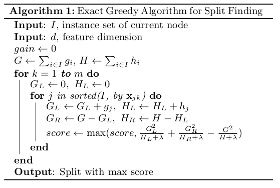
Finding split points with the greedy algorithm is a very effective algorithm, but for large datasets that cannot be loaded into memory at once, this method fails. In that case an approximate method is needed to find the split points.
The approximate method in fact proposes candidate split points according to the percentiles of the feature distribution. The continuous features are then mapped into the buckets divided by the candidate points, specifically as follows:
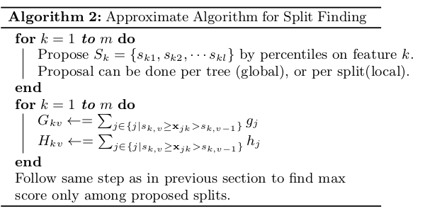
Here Global means the candidate split points are given before learning each tree, while Local means the candidate split points are given before each split
Weighted quantile sketch
In the approximate branching above, one important step is the selection of candidate points. Suppose the set $D_k=\\{(x_{1k},h_1),(x_{2k},h_2)\cdots(x_{nk},h_n)\\}$ represents the values of the k-th feature together with the statistics of their second derivatives. Define a rank function $r_k: \ R \rightarrow [0,+\infty)$:
$$ r_k(z) = \frac{1}{\sum_{(x,h) \in D_k}h}\sum_{(x,h) \in D_k, x \lt z}h \tag{10} $$This represents the proportion of instances in the sample whose corresponding feature value is less than z. Our goal is to find the optimal split points $\\{s_{k1},s_{k2},\cdots,s_{kl}\\}$, which can be done with:
$$ \vert r_k(s_{k,j})-r_k(s_{k,j+1})\vert \lt \epsilon, \ s_{k1}=min_i x_{ik}, s_{kl}=max_i x_{ik} \tag{11} $$Here $\epsilon$ is an approximation factor; roughly $\frac{1}{\epsilon}$ candidate split points can be assumed. Each data point here has a weight $h_i$.
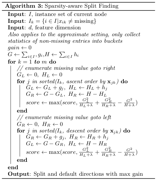
Sparsity-aware split finding
This part mainly deals with missing values in the samples. The method is to consider assigning the missing values to the left and right branches separately, and to pick the side with the larger gain, specifically as follows:
Cache access patterns
To speed up model computation, cache access patterns can be used, specifically as follows:
- For the greedy split-search algorithm: a cache-aware prefetching algorithm is used to alleviate memory access problems. That is, an internal buffer is requested for each thread, storing gradient statistics, and the accumulation is performed in small batches.
- For the approximate split-search algorithm: an appropriate block size is used to alleviate memory access problems. A block that is too small gives each thread little work and low efficiency; a block that is too large causes cache misses. It is usually set to $2^{16} \ examples \ per \ block$.
Note
The means by which Xgboost prevents overfitting:
- Adding a regularization term, that is, $\Omega(f)$ in the objective function
- Shinkage: after each iteration, the weights on the leaf nodes are multiplied by this coefficient, mainly to dampen the influence of each tree and leave more room for learning later on
- Column subsampling: similar to random forest, it supports feature subsampling, which prevents overfitting while reducing computation