The previous post mentioned an efficient tree ensemble algorithm, the Xgboost model, but its efficiency is still low when dealing with data that has a large feature dimension and a large number of samples. Compared with models such as GBDT and Xgboost, the Lightgbm model open-sourced by Microsoft uses a variety of techniques to reduce the amount of data and the number of features, which greatly speeds up training while keeping accuracy.
How to do
To reduce the impact of a large number of instances and a high feature dimension on model training, a natural idea is to reduce the number of data instances and the feature dimension. The schemes adopted by the Lightgbm model are Gradient-based One-Side Sampling (GOSS) and Exclusive Feature Bundling (EFB), respectively.
GOSS
This is essentially a sampling method. Microsoft found in experiments that if an instance has a small gradient, its contribution to model training is also small, because a small gradient means that the sample has already been trained well. GOSS keeps the samples with large gradients, randomly selects samples with small gradients, and compensates them with a constant weight. In this way, GOSS pays more attention to under-trained samples while not changing the original distribution too much. The related algorithm is shown below:
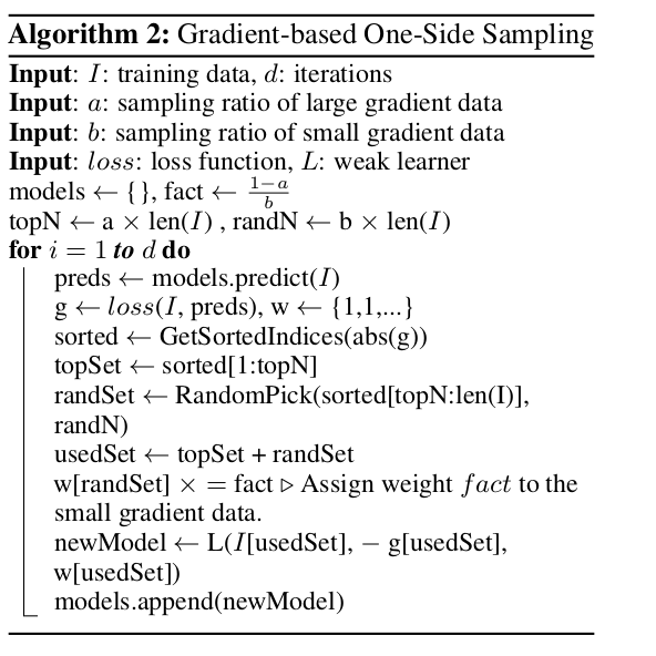
Specifically, GOSS first sorts samples by the absolute value of their gradients (from largest to smallest) and takes the first $a \times 100\%$ of the samples. Then it randomly selects $b \times 100\%$ of the remaining samples. After that, GOSS amplifies each sample with a small gradient by a constant weight (usually $\frac{1-a}{b}$).
EFB
Next comes the problem of reducing the feature dimension. In fact, we can notice that data with high-dimensional features is usually sparse, and in a sparse feature space many features are mutually exclusive, so we can bundle these exclusive features into a single feature. The specific algorithm is as follows:
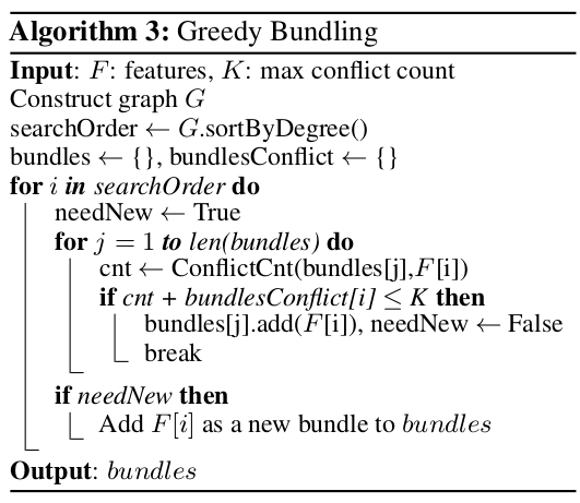
First we build a weighted graph, where the weight of an edge represents the amount of conflict between the two connected features (that is, the degree to which they are not mutually exclusive). Then the features are sorted in descending order by degree. Finally we traverse the sorted feature sequence and check whether a feature can be added to an existing bundle (determined by the amount of conflict); if not, a new bundle is created.
The above approach is indeed effective, but it is still unsatisfactory when the number of features is large. We can sort the features by their non-zero values to obtain the feature sequence, which avoids building the feature graph.
The features have now been placed into bundles, and the next step is to merge the features within the same bundle. The key here is that the original feature values can be distinguished from the bundle, because histogram-based algorithms store discrete bins rather than continuous feature values. This can be achieved by using offsets. Details are as follows:
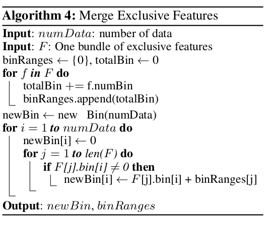
See the paper below for the detailed mathematical derivation
Reference
LightGBM: A Highly Efficient Gradient Boosting Decision Tree