Today’s deep neural networks have already become fully capable, especially in the vision field where they have approached or even surpassed human visual ability, and behind these deep learning networks there is always a basic framework, namely the convolutional neural network (CNN). CNN is mainly applied in the field of computer vision, so here I will briefly introduce the classic CNN model AlexNet. AlexNet was proposed by Alex Krizhevsky et al. in 2012. Although the model is rather rare nowadays (most people use resnet or something similar), it performed very well in the object detection field at the time and laid the foundation for other later CNN frameworks.
Introduction
In order to learn to recognize several thousand object categories from millions of images, Krizhevsky et al. built a model with strong learning ability, while taking into account that the enormous complexity of some object recognition tasks cannot be solved by enlarging the dataset, but requires a certain amount of prior knowledge to supplement the model. The capacity of a convolutional neural network model can be controlled through depth and width, and it can also accurately capture the two properties of natural images, namely statistical stationarity and locality of pixel regions, so using a CNN for image recognition is a good choice.
Basic framework
No more rambling, here is the screenshot:
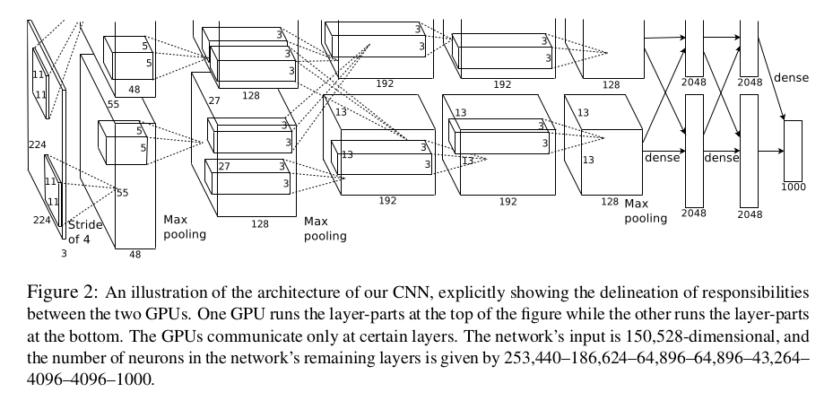
This framework contains 8 learning layers (5 convolution layers and 3 fully connected layers). Due to the limited GPU memory, the authors ran it on two GPUs and finally merged the computed data together, which is in fact a grouped convolution operation. In the model, the kernels of the second, fourth and fifth convolution layers are only connected to the previous convolution layer on the same GPU, while the third convolution layer is connected to all kernels of the second convolution layer. The response normalization layers come after the first and second convolution layers. Max pooling layers come after the response normalization layers and after the fifth layer, and the ReLU activation function is applied in every convolution layer and fully connected layer. The objective of the model is to maximize the multinomial logistic regression objective function. The following explains some special tricks used by the model.
Activation function
In 2012, the activation functions most used in neural networks were $f(x) = tanh(x)$ or $f(x) = (1+e^{-x})^{-1}$, but the authors adopt the now widely used ReLU activation function ($f(x) = max(0,x)$), which is a non-saturating nonlinearity; its descent is faster than that of the previous two saturating nonlinear functions, which made deep convolutional neural networks several times more efficient in training with the ReLU activation function.
Non-saturating nonlinear function: “nonlinear” simply means nonlinear as usually understood, while “non-saturating” means that as the variable x tends to infinity, the value of the function also tends to infinity.
Local response normalization
ReLUs have a very good property, namely that they do not require input normalization to prevent them from saturating. But the authors still use the following normalization:
$$ b^i_{x,y} = \frac{a^i_{x,y}}{\left(k+\alpha\sum^{min(N-1,i+n/2)}_{j=max(0,i-n/2)}{(\alpha^j_{x,y})^2}\right)^{\beta}} $$where $b^i_{x,y}$ denotes the normalized activation of the responding neuron, $\alpha^i_{x,y}$ is the activation of the neuron at position $(x,y)$ produced by applying kernel $i$ and the ReLU nonlinearity, $N$ is the total number of kernels in the layer, and the summation runs over the kernel maps at the same spatial position. The order of the kernel maps is arbitrary and is decided only at the start of training; this scheme implements a form of lateral inhibition, creating competition for large activations among the neuron outputs computed with different kernels.
As for the choice of hyperparameters, the authors chose: $k=2$, $n=5$, $\alpha=10^{-4}$ and $\beta=0.75$.
Overlapping pooling
The pooling layers in a CNN summarize the outputs of neighboring groups of neurons in the same kernel map. The usual pooling operation is done through adjacent pooling units; specifically, a pooling layer can be seen as consisting of merging cells spaced $S$ pixels apart, each summarizing a $Z \times Z$ neighborhood centered on that cell. If we let $S = Z$, we get the traditional convolutional neural network pooling operation; for $S < Z$ we get overlapping pooling. The authors chose the parameters $S = 2$ and $Z = 3$. Models with overlapping pooling are slightly harder to overfit during training.
Reducing overfitting
Data augmentation
A simple and common way to reduce overfitting is data augmentation to enlarge the dataset. In the paper, the augmentation methods used by the authors are mainly image translation and horizontal reflection, and altering the intensities of the RGB channels of the training images.
First, image translation and horizontal reflection: the authors randomly extract $224 \times 224$ patches from $256 \times 256$ images together with the corresponding horizontally reflected patches, and then train the model on this data. At prediction time, the model uses five $224 \times 224$ patches (the four corners and the center) together with their horizontally reflected patches, that is, 10 patches in total, and finally the predictions are combined through a $softmax$ layer to obtain the final prediction.
As for altering the intensities of the RGB channels of the training images, the authors apply $PCA$ to the set of RGB pixel values across the training set. For each training image, multiple found principal components are added, with magnitudes proportional to the corresponding eigenvalues multiplied by a random variable drawn from a Gaussian with mean 0 and standard deviation 0.1. So for each RGB pixel value $I_{xy} = [I^R_{xy},I^G_{xy},I^B_{xy}]$, the following values are added:
$$ [\mathbf{p}_1,\mathbf{p}_2,\mathbf{p}_3][\alpha_1\lambda_1,\alpha_2\lambda_2,\alpha_3\lambda_3]^T $$where $\mathbf{p}_i$ and $\lambda_i$ are the $i$th eigenvector and eigenvalue of the $3 \times 3$ covariance matrix of the RGB pixel values, and $\alpha_i$ is the random variable mentioned above; for all pixels of a particular training image each $\alpha_i$ is drawn only once, until that image is used again for training, at which point the $\alpha_i$ are drawn again. This scheme roughly captures the property of natural images that object identity is invariant to changes in the intensity and color of illumination.
Dropout
With a certain probability (the authors chose 0.5), the output of a hidden layer neuron is set to 0. Such a neuron then contributes nothing to the forward propagation and is also unaffected by error backpropagation, that is, the neural structure changes. This technique reduces the complex co-adaptation of neurons, because a neuron cannot rely on particular other neurons. The dropout probability of 0.5 chosen by the authors is the geometric mean of the predictive distributions produced by an exponential number of dropout networks. The dropout operation roughly doubles the number of iterations needed for the model to converge.
Some training details
The optimization method is SGD, with a batch size of 128, a momentum parameter of 0.9 and a weight decay parameter of 0.0005. The authors found that a small amount of weight decay is important for the model’s learning. The weight update is as follows:
$$ \begin{aligned} \mathbb{v}_{i+1} & := 0.9\cdot\mathbb{v}_i-0.0005\cdot\epsilon\cdot\mathbb{\omega}_i-\epsilon\cdot\left\langle\frac{\partial{L}}{\partial{\mathbb{\omega}}}\vert_{\mathbb{\omega}_i}\right\rangle_{D_i} \\ \mathbb{\omega}_{i+1} & := \mathbb{\omega}_i+\mathbb{v}_{i+1} \end{aligned} $$where the partial derivative term of the first equation is the average over batch $i$ of the value at $w_i$ of the derivative of the loss on $D_i$ with respect to $w$, $i$ is the iteration index, $v$ is the momentum variable and $\epsilon$ is the learning rate.
The model weights are initialized with a Gaussian distribution of mean 0 and standard deviation 0.01, and the biases of the second, fourth and fifth convolution layers and of the fully connected hidden layers are initialized to the constant 1, which accelerates the early stage of learning by providing positive input to the ReLUs; the remaining neuron biases are set to 0. For all layers the authors use the same learning rate (0.01) and adjust it during training: when the validation error rate stops decreasing under the current learning rate, the learning rate is divided by 10, and training is stopped after the learning rate has been reduced three times.
In short, the AlexNet model achieved quite good results in the 2012 ImageNet competition, where the Top-5 error rate was reduced to $15.3\%$. This model can be said to be a very classic model for getting started in the deep learning vision field, and many of the tricks used in it have also found good use in the subsequent development of models.
Reference
This post refers to the paper published by Alex Krizhevsky et al. in 2012:
ImageNet Classification with Deep Convolutional Neural Networks