VGG (Visual Geometry Group) is another classic convolutional neural network model after AlexNet. It won second place in the 2014 ILSVRC competition (first place went to GoogleLeNet), and the variants used most often in work and personal projects are VGG16 and VGG19, where 16 and 19 denote the number of layers in the network. Following on from the AlexNet model discussed previously, this post analyzes the VGG model.
Basic architecture
The training input images are $224 \times 224$ RGB images, and the only preprocessing is subtracting the mean RGB value of the training set from every pixel. The convolution layers use a kernel size of $3 \times 3$ with stride 1, and some convolution kernels use a $1 \times 1$ size; the max pooling layers use a kernel size of $2 \times 2$ with stride 2. Of the three fully connected layers at the end, the first two have 4096 channels, followed by a $softmax$ layer; the hidden layer activation function is $ReLU$, and the LRN local response normalization used in AlexNet is not used. The detailed structure is shown in the table below:
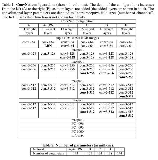
All the networks above follow the basic architecture described earlier, and the only difference is the depth of the network (also shown in the table). As for the width of the network layers, it starts at $64 \times 64$ from the first layer, then doubles after each max pooling layer until reaching $512 \times 512$. The table below shows the number of parameters of each network model.
Some tricks
When building the network, the authors used only small $3 \times 3$ convolution kernels with stride 1 throughout: two stacked $3 \times 3$ convolution layers (with no pooling in between) have the same receptive field as a $5 \times 5$ convolution layer, and likewise three stacked $3 \times 3$ convolution layers are equivalent to a $7 \times 7$ convolution layer.
Replacing large-kernel convolution layers with stacks of small-kernel convolution layers has the following main advantages:
- It uses several nonlinear rectification layers instead of a single one, which strengthens the expressive power of the model;
- It reduces the parameter size of the model
This operation can also be seen as regularizing the original convolution layers, forcing them to be decomposed through small kernels while introducing nonlinearity; the rectification function also brings in extra nonlinearity.
Training uses mini-batch gradient descent to optimize the multinomial logistic regression objective (momentum 0.9, batch size 256); weight decay regularization is used with an $L_2$ regularization coefficient of $5 \times 10^{-4}$; Dropout regularization is used in the first two fully connected layers (with the Dropout parameter set to 0.5); the learning rate is initialized to $10^{-2}$, and similar to the AlexNet model, the learning rate is decreased once whenever the validation set score stops improving, and training stops after three decreases or when the number of iterations reaches 370K (that is, 74 epochs).
After some experimentation, the authors initialize the weights with a normal distribution of mean 0 and variance 0.01, and initialize the biases to 0. To accommodate $224 \times 224$ input images, the authors randomly crop from the rescaled image in each epoch, and also apply random horizontal flipping and random RGB color shifting.
Handling of training image size
Let $S$ be the smallest side of the isotropically rescaled training image (this parameter is also referred to as the scale of the training image). In principle $S$ should be no smaller than 224 (since the input size is $224 \times 224$); when $S = 224$ the crop covers the entire image, and when $S >> 224$ the crop corresponds to a small region of the original image, which may contain small objects or parts of objects. The authors propose two ways to set the training scale $S$. The first is fixed-scale training, which corresponds to training at a single scale; the second is multi-scale training, where each training image is rescaled individually by randomly sampling $S$ from a range $[S_{min}, S_{max}]$ (the authors use $[256, 512]$). Since different objects have different sizes, this approach can capture objects better, and it can also be viewed as augmenting the training set through scale jittering.
Handling of the test set
Let $Q$ be the test scale (the authors found experimentally that the test scale need not be the same as the training scale). The fully connected layers of the model are converted into convolution layers (the first FC layer becomes a $7 \times 7$ convolution layer and the last two FC layers become $1 \times 1$ convolution layers), and the modified model is applied directly to the whole uncropped image (including the augmented versions of the image). The result is a class score map (with as many channels as classes), which is then spatially averaged (summed) to obtain a fixed-size class score vector for the image; finally the $softmax$ class posteriors of the original and flipped images are averaged to obtain the final score for the image.
Since the fully convolutional network is applied to the whole image, multi-crop evaluation is not needed at test time. However, multi-crop evaluation can complement the dense evaluation of the test set, because when the convolutional network is applied to crops the convolution feature maps are zero-padded, whereas dense evaluation over the test set pads the feature maps with neighboring pixel values (this comes from the convolution and pooling operations), which provides more contextual information.
See the original paper for the concrete models and experimental results
Reference
This post refers to the paper published by Karen Simonyan et al. in 2015:
VERY DEEP CONVOLUTIONAL NETWORKS FOR LARGE-SCALE IMAGE RECOGNITION