First of all, happy Teachers’ Day to all teachers, and thank you for your spirit of giving roses to others with a lingering fragrance on your hands. Then, after almost a month, I have rolled back to update the blog again; before that I was busy with joining the company, hoping to fit into the company’s development work as soon as possible, so I was “busy” for a month. Next let us continue with the introduction of classic image recognition network models. In previous posts we already introduced the AlexNet and VGG networks, both of which pushed the depth of neural networks of that time to the extreme, and subsequent neural network models basically performed no better. This is because as the network gets deeper, during error backpropagation the weights of the earlier network layers basically do not get updated and stay around some fixed value. In 2015, Kaiming He proposed a shortcut connection that propagates the error to the earlier network layers, greatly improving network performance. Below is a brief analysis of the ResNet network.
Shortcut connections
Increasing the number of neural network layers should in theory give a better performing model, but the existence of vanishing gradients limits how deep the network can go. For this reason, Kaiming He proposed a network building block that solves the problem of gradients not being able to propagate to the bottom layers of the network, namely the shortcut connection. The basic structure is shown below:

This structure is in fact a residual network. Here $x$ denotes the input of this building block and $\mathcal{H}(x)$ denotes the mapping function of the building block. Assuming a multi-layer nonlinear network structure can fit any complex function, that is, this structure can fit the residual function $\mathcal{H}(x)-x$, it is better to fit the residual function $\mathcal{F}(x) := \mathcal{H}(x)-x$ than to fit the original mapping function $\mathcal{H}(x)$, because fitting the original function still cannot avoid the vanishing gradient phenomenon, and from the figure we can see that implementing the residual function is very simple.
There is a very important component in the shortcut connection, namely the $Identity \ Mapping$; the building block in the figure above can be written as: $y = \mathcal{F}(x,\{\mathcal{W}_i\})+x$, where $x$ and $y$ denote the input and output of the block respectively (before the activation function), and $\mathcal{F}(x,\{\mathcal{W}_i\})$ denotes the function mapping learned by the residual block. Expanding the figure above gives: $\mathcal{F} = W_2\sigma(W_1x)$, where $\sigma$ denotes the $ReLU$ activation function and the bias values are ignored here. This connection introduces no additional parameters and does not increase the computation of the model. There is one point to note: $x$ and the output of $\mathcal{F}$ must have the same dimension; if they do not, the dimension can be matched with a linear projection $W_s$: $y = \mathcal{F}(x,\{\mathcal{W}_i\})+W_sx$.
Basic structure
The authors set up three groups of network models for the $ImageNet$ dataset, taking these as examples to explain the structure of $ResNet$
Plain convolutional neural network
The design of the basic network mostly comes from the $VGG$ network; the convolution kernels of the convolution layers are basically $3 \times 3$ and follow the following two simple design principles:
- For network layers with the same output size, set the same number of convolution kernels;
- If the size of the feature map is halved, double the number of convolution kernels to reduce the computational complexity of each layer
For convolution layers with stride 2, the authors perform downsampling directly in that layer. The overall network ends with a global average pooling layer and a 1000-way fully connected layer with $softmax$. The network model has $34$ weight layers.
Convolutional neural network with residual blocks
It is modified from the plain neural network designed before by adding shortcut connections. Shortcut connections can be used directly when the dimensions before and after the connection are the same; for the case of different dimensions, there are the following two ways of handling it:
- Use zero padding to expand the dimension for matching, which introduces no additional parameters;
- Use a $1 \times 1$ convolution kernel to expand the dimension
The concrete structure figure is as follows:
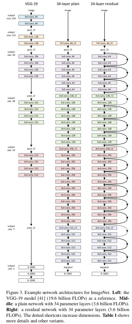
The left side is the $VGG$ network (used as a reference), the middle is the plain convolutional neural network, and the right is the convolutional neural network with residual blocks; the dashed shortcut connections indicate that the dimension is increased during the connection.
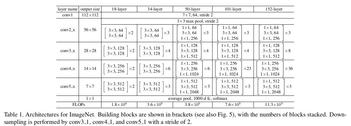
In later experiments the authors also adopt many variants of the $ResNet$ network, with the concrete structure as follows:
Identity Mapping
Not long after publishing the $ResNet$ paper, the authors published a paper on the mathematical principles of the $Identity \ Mapping$ in the shortcut connections of the $ResNet$ network to further confirm the reliability of this model. Here is a rough analysis.
A residual block can be written in the following form:
$$ \begin{aligned} y_l & = h(x)+\mathcal{F}(x_l,\mathcal{W}_l) \\ x_{l+1} & = f(y_l) \end{aligned} $$where $x_l$ and $x_{l+1}$ are the input and output of the $l$-th residual block, $\mathcal{F}$ is the residual function and $f$ is the $ReLU$ activation function, with $\mathcal{W}_l$ defined as follows:
$$ \mathcal{W}_l=\{W_{l,k}\vert 1\le k\le K\} $$$l$ is the weight of the $l$-th block (including the bias values) and $K$ is the number of network layers in the residual block.
To prove the correctness of the $Identity \ Mapping$ choice, the authors made several assumptions here, and to simplify the analysis they also unified the $f$ function (all being $Identity \ Mapping$), so that $x_{l+1}=y_l$.
Let $h(x_l)=x_l$, that is, $Identity \ Mapping$
From the assumption we obtain:
$$ x_{l+1} = x_l+\mathcal{F}(x_l, \mathcal{W}_l) $$Recursively:
$$ \begin{aligned} x_{l+2} & = x_{l+1}+\mathcal{F}(x_{l+1},\mathcal{W}_{l+1}) \\ & = x_l+\mathcal{F}(x_l,\mathcal{W}_l)+\mathcal{F}(x_{l+1},\mathcal{W}_{l+1}) \\ & = \dots \end{aligned} $$which simplifies to:
$$ x_L = x_l+\sum_{i=1}^{L-1}\mathcal{F}(x_i,\mathcal{W}_i) $$This form has two benefits:
- The feature $x_L$ of a residual block at any depth can be expressed by any shallow residual block $l$ plus the residual terms $\sum_{i=1}^{L-1}\mathcal{F}$, that is, the model is in a residual fashion between any blocks $L$ and $l$;
- For a residual block $L$ at any depth, the equation $x_L = x_0+\sum_{i=0}^{L-1}\mathcal{F}(x_i,\mathcal{W}_i)$ sums the outputs of all preceding residual functions, unlike the matrix-vector product of ordinary network models
(Addition: the matrix-vector product form of an ordinary network model is: $x_L=\prod_{i=0}^{L-1}\mathcal{W}_ix_0$)
This form also performs very well in backpropagation. Let $\epsilon$ be the loss function; then:
$$ \begin{aligned} \frac{\partial{\epsilon}}{\partial{x_l}} & = \frac{\partial{\epsilon}}{\partial{x_L}}\cdot\frac{\partial{x_L}}{\partial{x_l}} \\ & = \frac{\partial{\epsilon}}{\partial{x_L}}\left(1+\frac{\partial{}}{\partial{x_l}}\sum_{i=1}^{L-1}\mathcal{F}(x_i,\mathcal{W}_i)\right) \end{aligned} $$Here $\frac{\partial{\epsilon}}{\partial{x_L}}$ propagates directly without passing through weight layers, while the other term propagates through weight layers. For $\frac{\partial{}}{\partial{x_l}}\sum_{i=1}^{L-1}\mathcal{F}(x_i,\mathcal{W}_i)$, the value over a $minibatch$ is not always -1, that is, vanishing gradients do not occur (because $\frac{\partial{\epsilon}}{\partial{x_l}}$ will not be zero).
Let $h(x_l)=\lambda_lx_l$, where $\lambda_l$ is a modulation parameter
Likewise from the assumption we obtain $x_{l+1}=\lambda_lx_l+\mathcal{F}(x_{l},\mathcal{W}_{l})$, and recursively
$$ x_L=(\prod_{i=1}^{L-1}\lambda_i)x_l+\sum_{i=1}^{L-1}(\prod_{j=i+1}^{L-1}\lambda_j)\mathcal{F}(x_i,\{\mathcal{W}_i\}) $$Simplification gives the following:
$$ x_L=(\prod_{i=l}^{L-1}\lambda_i)x_l+\sum_{i=1}^{L-1}\hat{\mathcal{F}}(x_i,\mathcal{W}_i) $$where $\hat{\mathcal{F}}(x_i,\mathcal{W}_i)$ absorbs the scalar. Backpropagating the formula above gives:
$$ \frac{\partial{\epsilon}}{\partial{x_l}} = \frac{\partial{\epsilon}}{\partial{x_L}}\left((\prod_{i=l}^{L-1}\lambda_i)+\frac{\partial{}}{\partial{x_l}}\sum_{i=l}^{L-1}\hat{\mathcal{F}}(x_i,\mathcal{W}_i)\right) $$When the network is very deep ($L$ is large), if $\lambda_i \lt 1$ for all $i$, the factor $\prod_{i=l}^{L-1}\lambda_i$ grows explosively; if $\lambda_i \gt 1$ for all $i$, the factor $\prod_{i=l}^{L-1}\lambda_i$ becomes very small or even zero — both of which hinder the network’s learning.
Choosing the activation function
Above we argued for the importance of $Identity \ Mapping$, and this was based on an important assumption, namely that the activation function $f$ is an $Identity \ Mapping$. So next the authors discuss the case where the activation function takes other forms. The concrete detail figures are as follows:
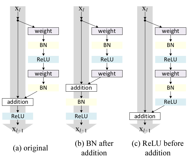
In the figure, $a$ is the reference block and keeps the original structure, with $ReLU$ as the only activation; $b$ places the $BN$ layer after the addition operation, that is, the activation includes the $BN$ layer and $ReLU$; the authors’ experiments show that this structure is less expressive than the original one, because the $BN$ layer in this structure affects the information flow; $c$ places $ReLU$ before the addition operation, so the activation becomes an $Identity \ Mapping$, but this makes the output of the function $\mathcal{F}$ non-negative, whereas intuitively the function $\mathcal{F}$ should take values in $(+\infty, -\infty)$, so the result is that the forward-propagated signal of the residual block increases monotonically, which affects the expressiveness of the model.
Improving the residual block
For the original structure we have:
$$ \begin{aligned} y_l & = h(x_l)+\mathcal{F}(x_l,\mathcal{W}_l) \\ x_{l+1} & = f(y_l) \end{aligned} $$For the next block we have:
$$ \begin{aligned} y_{l+1} & = h(x_{l+1})+\mathcal{F}(x_{l+1},\mathcal{W}_{l+1}) \\ & = x_{l+1}+\mathcal{F}(x_{l+1},\mathcal{W}_{l+1}) \\ & = f(y_l)+\mathcal{F}(f(y_l),\mathcal{W}_{l+1}) \end{aligned} $$From the formula we can see that the function $x_{l+1}=f(y_l)$ affects both this block and the next block.
The authors propose an asymmetric structure to solve this problem, with the concrete structure as follows:
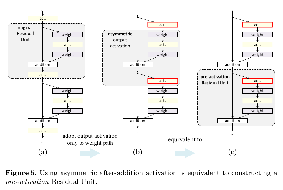
expressed as:
$$ x_{l+1} = x_l+\mathcal{F}(\hat{f}(x_l), \mathcal{W}_l) $$From the figure we can also see that $post-activation$ and $pre-activation$ are equivalent; the mathematical expression is similar to $x_L = x_l+\sum_{i=1}^{L-1}\mathcal{F}(x_i,\mathcal{W}_i)$, so the backward propagation form is similar too, that is, there is no vanishing or exploding gradient, and the activation function in the structure above takes the $Identity \ Mapping$ form.
Choosing the position of the activation function after the improvement
For the position of the activation function in the improved residual block, the authors considered two structures, as follows:
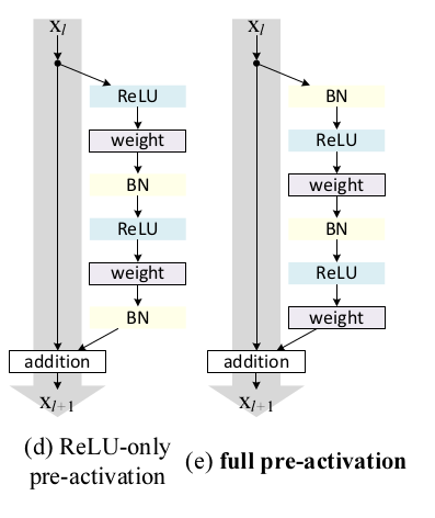
Experiments show that the structure shown in figure $e$ achieves better performance than the others, mainly for two reasons:
- The activation function is an $Identity \ Mapping$. The authors found experimentally that the closer $h(x_l)$ and the activation function $f$ in the shortcut connection block are to $Identity \ Mapping$, the better the model’s representational ability;
- Using a $BN$ layer in the pre-activation improves the regularization ability of the model. Although the original structure also has a $BN$ layer for regularization, the value passed through the shortcut connection is added afterwards, so the output of the whole block is not regularized, whereas pre-activation regularizes both the input and the output of the block.
This structure is also easy to optimize: the activation function $f=ReLU$ of the original block affects signal propagation in the negative case, and this effect strengthens as the number of residual blocks grows. The activation function of the improved block uses $Identity \ Mapping$, which can propagate the error directly to the next layer.
Reference
This post refers to the two papers published by Kaiming He in 2015 and 2016: