Ha, since I happen to have some free time these days, let me quickly summarize the RCNN series papers I read before; this is the second post in the series. The author Ross Girshick could not stand how slowly the model he had proposed earlier (RCNN) ran, so he proposed an improved model (Fast RCNN). Below is a brief analysis of that model.
The slowness of RCNN
Compared with image recognition tasks, object detection is considerably harder because of the extra step of localizing the object positions. There are two main problems to solve: one is that the model needs a large number of object candidate boxes; the other is that these candidate boxes only roughly provide the approximate positions of the objects, so the model has to perform a regression operation. $RCNN$ is a multi-stage training model. The $RCNN$ model first fine-tunes a convolutional neural network on the object candidate boxes using a log loss, then passes the resulting feature maps to $SVM$s for object classification; these $SVM$s replace the $softmax$ layer that would otherwise need fine-tuning. In the third training stage the model learns bounding box regression. For training the $SVM$s and the bounding box regression, $RCNN$ writes the features of every object candidate box to disk, which undoubtedly costs an enormous amount of time and space. Secondly, the speed of object recognition is too slow: on a GPU, recognizing an image takes about 47 seconds per image. Another important reason for the slowness of $RCNN$ is that the model does not share the computation of the convolution layers.
Basic structure
$Fast \ RCNN$ is a single-stage training model. It takes the whole image and a set of candidate boxes as input; the model first extracts features from the whole image with a set of convolution layers and max pooling layers, then, on the extracted feature map, uses a $RoI \ pooling$ layer to extract a fixed-length feature vector for each candidate box, and then feeds it into fully connected layers that finally split into two branches for object recognition and bounding box regression respectively. The concrete framework is as follows:
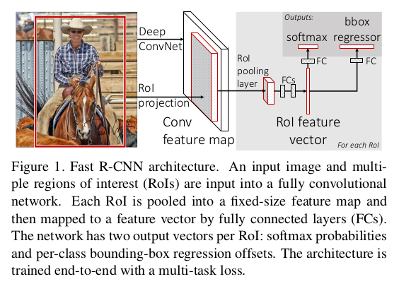
$RoI \ pooling$ divides an $h \times w$ $RoI$ region into sub-windows of $h/H \times w/W$, then applies $max \ pooling$ on each sub-window to output a fixed-length feature vector.
Pretraining and fine-tuning the network
For network initialization, the authors use three pretrained $ImageNet$ models and make the following changes:
- The last $max \ pooling$ layer of the original network is replaced by a $RoI \ pooling$ layer with the parameters $H \times W$ specified to match the size of the network’s first fully connected layer;
- The last fully connected network and $softmax$ layer of the original network are replaced by two branch networks;
- The original network is modified to have two inputs
The authors propose an efficient model training method that has the advantage of shared features. In $Fast \ Rcnn$ training, the $minibatch$ of stochastic gradient descent is sampled hierarchically: first $N$ samples are sampled, then $R/N$ $RoI$s are sampled from each sample. The $RoI$s coming from the same image share the computation and memory of the forward and backward passes.
The loss function used by the model is a multi-task loss function. $Fast \ RCNN$ has two output layers: one outputs the probabilities $p=(p_0,\dots,p_K)$ over $K+1$ classes for each $RoI$, and the other outputs the bounding box regression offsets $t^k=(t_x^k,t_y^k,t_w^k,t_h^k)$ over the $K$ classes. Each $RoI$ is labeled with a ground truth class $u$ and a ground truth bounding box $v$ of that class. The authors use a multi-task loss function $L$ on each labeled $RoI$ to jointly train classification and bounding box regression:
$$ L(p,u,t^u,v) = L_{cls}(p,u)+\lambda[u \ge 1]L_{loc}(t^u,v) $$where $L_{cls}(p,u)=-logp_u$ is the log loss, and the second loss term is composed of the ground truth regression box $v=(v_x,v_y,v_w,v_h)$ and the predicted regression box $t^u=(t_x^u,t_y^u,t_w^u,t_h^u)$; $L_{loc}$ ignores background $RoI$ classes, so for bounding box regression we have:
$$ L_{loc}(t^u,v) = \sum_{t \in \{x,y,w,h\}} smooth_{L_1}(t_i^u-v_i) $$And the $smooth$ function is:
$$ smooth_{L_1}(x) = \begin{cases} 0.5x^2 &\text{if $\vert x \vert\lt 1$} \\ \vert x \vert-0.5 \ &\text{otherwise} \end{cases} $$Using the $L_1$ loss here is less sensitive than the $L_2$ loss used by $RCNN$. The hyperparameter $\lambda$ in the multi-task loss function controls the balance between the two individual loss functions. In the paper’s experiments the authors normalized the ground truth bounding boxes (to have mean 0 and variance 1), and chose the hyperparameter in the loss function to be 1.
I will not go into the sampling of the $minibatch$ in detail here; see the authors’ paper. Next let me talk about the backward propagation of the $RoI \ pooling$ layer. Let $x_i \in R$ be the i-th input of $RoI \ pooling$ and $y_{rj}$ be the j-th output of the r-th $RoI$; then the computation of $RoI \ pooling$ can be written as
$$ y_{rj}=x_{i^*(i,j)} $$where $i^*(r,j)=argmax_{i^\prime\in R(r,j)}x_i^\prime$, and $R(r,j)$ is the index set of the input sub-window. A single $x_i$ may correspond to several different outputs $y_{rj}$. Its backward propagation form is:
$$ \frac{\partial{L}}{\partial{x_i}} = \sum_r\sum_j[i=i^*(r,j)]\frac{\partial{L}}{\partial{y_{rj}}} $$In the backward propagation of the $RoI$ pooling layer, the gradient of the loss function $L$ with respect to the input node $x_i$ is the accumulation of the gradients of $L$ with respect to the outputs $y_{rj}$ of each possible candidate region $r$ ($x_i$ is selected as the maximum by the j-th output of the r-th candidate region). The indicator function in the formula above is specifically:
$$ [i=i^*(r,j)] = \begin{cases} 1, & i=i^*(r,j) \ge 1 \\ 0, & \text{otherwise} \end{cases} $$For whole-image classification, the time consumed by the fully connected layers is less than that of the convolution layers, but in this model a large number of $RoI$s are used for object detection, so the computation of the fully connected layers accounts for roughly $50\%$ of the overall model. So the authors apply $SVD$ truncation to the large fully connected layers. A fully connected layer can be parameterized by a weight matrix $W$ of size $u \times v$, and applying $SVD$ to this matrix gives:
$$ W \approx U\Sigma_tV^T $$where $U$ is the $u \times t$ left singular matrix of $W$, $\Sigma_t$ is the $t \times t$ diagonal matrix of singular values of $W$, and $V$ is the $v \times t$ right singular matrix of $W$. This simple compression operation yields a good speedup.
About the model
Later in the paper the authors also discuss the model in the form of questions. The first is the multi-task loss: it avoids designing a pipelined sequential training model, and the experimental results also show that this design performs better than multi-stage training. The $Fast \ RCNN$ model also replaces the $SVM$s of the $RCNN$ model with a $softmax$ layer; the $softmax$ layer introduces competition between classes when predicting scores for $RoI$s, so the final result is better than with $SVM$s. Finally, one point to note: more candidate boxes do not mean better model performance — the authors found experimentally that sparse object candidate boxes can improve model performance.
Reference
This post refers to the following paper: