This feeling of posting several articles in a row is very exciting, very refreshing. Without further ado, as the title says, this is a faster and stronger object detection algorithm, and it also comes from Ross Girshick… Honestly, this guy spent several papers in a row criticizing the models he had written before — impressive. Faster Rcnn adopts an efficient algorithm to generate candidate boxes, and also introduces the concept of Anchor.
Basic structure
In $Fast \ RCNN$, the method of proposing candidate boxes was not discussed at all; $selective \ search$ was simply mentioned for choosing candidate boxes, and later this became the main reason for slowing the model down. In the $Faster \ RCNN$ model the authors made an improvement and proposed a new candidate box extraction method, namely $RPN$. Combined with this method, the running speed of the model was greatly improved, and the accuracy also improved. The rough structure of $Faster \ RCNN$ is as follows:
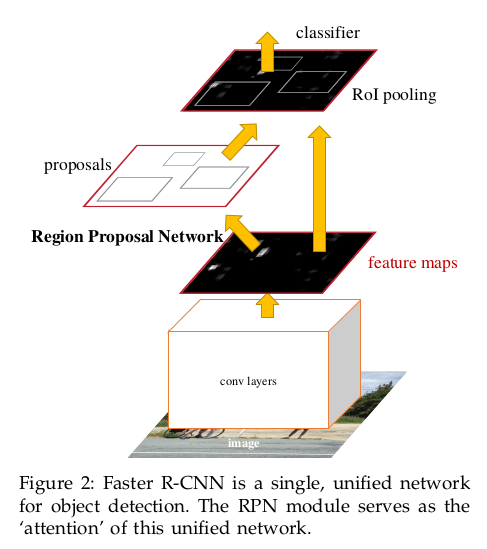
Its structure mainly consists of two parts: first a deep fully convolutional network used to generate candidate regions, and then the $Fast \ RCNN$ model used for classification and bounding box regression. $RPN$ is applied to the convolved feature maps.
Region Proposal Networks
The $RPN$ network takes an image of arbitrary size as input and outputs a set of object candidate boxes together with classification scores. To generate candidate regions, $RPN$ slides a small network over the convolutional feature map, and this small network takes an $n \times n$ window on the feature map as input. Each sliding window generates a low-dimensional feature, which is fed into two branches: a bounding box regression layer ($reg$) and a box classification layer ($cls$). The structure is roughly as follows:
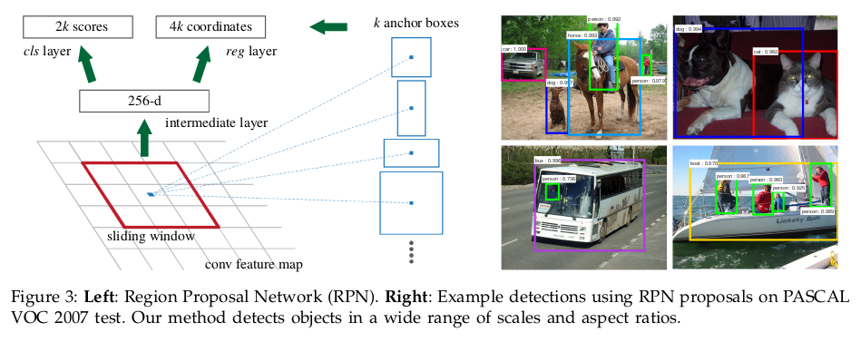
There is an important point here, namely the $Anchor$. At each sliding window position we need to predict multiple candidate boxes simultaneously; let the maximum number of candidate boxes per position be $k$, so the input of the $reg$ layer is $4k$ (encoding the coordinates of the candidate boxes) and the input of the $cls$ layer is $2k$ (that is, whether the candidate box is an object). The $Anchor$ is in fact the center of the sliding window, related to the scale and aspect ratio (my understanding is that the mapping of the current sliding window center onto the original pixel space is the $Anchor$). In the paper’s experiments, 3 scales and 3 aspect ratios were used, that is, 9 $anchor$s are generated per sliding window position; for a convolutional feature map of size $W \times H$, $WHK$ $anchors$ are generated in total. Compared with the previous image pyramids and feature pyramids, our multi-scale detection design based on $Anchors$ relies only on a single-scale image and feature map, and uses sliding windows over a single-size feature map.
$Anchor$ has another important property, namely translation invariance. If an object in an image is translated, the candidate region should be translated as well, and the same function can predict the candidate box at any position. This property also reduces the number of model parameters.
To train the $RPN$, the authors assign a binary class label to each $Anchor$. An $anchor$ is assigned a positive label in the following two cases:
- The candidate box with the highest $IoU$ with a ground truth instance;
- A candidate box with an $IoU$ above 0.7 with any ground truth instance
A candidate box with an $IoU$ below 0.3 is labeled negative, and $anchors$ with an $IoU$ between 0.3 and 0.7 do not participate in $RPN$ training. The training loss function is:
$$ L(\{p_i\},\{t_i\}) = \frac{1}{N_{cls}}\sum_iL_{cls}(p_i,p_i^*)+\lambda\frac{1}{N_{reg}}\sum_ip_i^*L_{reg}(t_i,t_i^*) $$where $i$ is the index of an $anchor$ within a $minibatch$ and $p_i$ denotes the probability that the $i$th $anchor$ is an object. $p_i^{\*}$ is the ground truth label indicator, equal to 1 when the $anchor$ is positive and 0 when it is negative. $t_i$ is the coordinate vector of the predicted box, and $t_i^{\*}$ is the coordinate vector of the ground truth instance. $L_{cls}$ is the log loss over the two classes; for the box regression loss, the following is used:
$$ L_{reg}(t_i,t_i^*)=R(t_i-t_i^*) $$where $R$ is the $smooth \ L_1$ function. The $p_i^*L_{reg}$ term in the formula above means that the regression loss is only computed when the $anchor$ is positive. The outputs of the $cls$ and $reg$ layers consist of $\{p_i\}$ and $\{t_i\}$, respectively.
The two losses are normalized by $N_{cls}$ and $N_{reg}$ respectively, with $\lambda$ controlling the balance. But the authors show experimentally that the model is not sensitive to $\lambda$ over a wide range, and that the normalization mentioned above is not essential and can be simplified.
Bounding box regression is done in the same way as in $RCNN$, and here the ground truth bounding boxes are also parameterized as $(t_x^*, t_y^*, t_w^*, t_h^*)$:
$$ \begin{aligned} t_x & = (x-x_a)/w_a \\ t_y & = (y-y_a)/h_a \\ t_w & = log(w/w_a) \\ t_h & = log(h/h_a) \\ t_x^* & = (x^*-x_a)/w_a \\ t_y^* & = (y^*-y_a)/h_a \\ t_w^* & = log(w^*/w_a) \\ t_h^* & = log(h^*/h_a) \end{aligned} $$Using the logarithm to represent the difference in width and height also has the effect of converging quickly when the difference is large and more slowly (to guarantee accuracy) when the difference is small.
Model training
For the detection network the authors use $Fast \ RCNN$. During training the $RPN$ and $Fast \ RCNN$ are trained separately. There are three methods for training such a network with shared features:
- $Alternating \ training$. First the $RPN$ is trained, then the candidate boxes are used to train $Fast \ RCNN$; after being fine-tuned by $Fast \ RCNN$ the network is used in turn to initialize the $RPN$, and this process can be iterated.
- $Approximate \ joint \ training$. This method fuses $RPN$ and $Fast \ RCNN$ into a single network for training. In each $SGD$ iteration, the forward pass through the $RPN$ does not change its parameters and precomputed candidate boxes are used to train $Fast \ RCNN$, while the backward pass proceeds normally. For the backward pass of the shared convolution layers, the propagated information comes from both the $RPN$ loss and the $Fast \ RCNN$ loss. This method ignores the derivative information with respect to the candidate box coordinates.
- $Non-approximate \ joint \ training$. This method fixes the flaw of the previous one and includes the candidate box coordinate information. It requires a $RoI \ pooling$ layer that is differentiable with respect to the box coordinates, which can be solved with a $RoI \ warping$ layer.
The authors adopt $4-step \ Alternating \ Training$, with the four steps as follows:
- Train the $RPN$, initializing the network with an $ImageNet$ pretrained model and fine-tuning it end to end with the region proposal loss;
- Train $Fast \ RCNN$ using the candidate boxes generated in the first step; this network is also initialized with the $ImageNet$ pretrained model. Up to this point the two networks do not share the computation of the convolution layers;
- Train the $RPN$ using the detection network, while freezing the convolution layers and only adjusting the layers belonging to the $RPN$ model;
- Keeping the convolution layers frozen, fine-tune the layers belonging to the $Fast \ RCNN$ model. In this way both networks share the computation of the convolution layers.
Both $Faster \ RCNN$ and $Fast \ RCNN$ belong to the $two \ stage$ algorithms. The characteristic of such algorithms is that the algorithm first generates a series of candidate boxes as samples, and then performs classification and regression on these boxes. This gives high accuracy but slow speed. The single-stage algorithms ($one \ stage$) instead turn the object localization problem into a regression problem, gaining considerably more speed but losing accuracy.
Reference
There are many details about the $Faster \ RCNN$ model that are not mentioned here; refer to the original paper and the related code open-sourced by the authors.
This post is mainly based on the following articles:
Faster R-CNN: Towards Real-Time Object Detection with Region Proposal Networks