First of all, I must congratulate the People’s Republic of China on its 70th anniversary. To celebrate the arrival of the National Day holiday, I took the time to go through the SSD object detection model and then struck while the iron was hot to update the blog… The biggest difference between the SSD algorithm and the previous RCNN series algorithms is that it is single-stage, whereas the RCNN series is multi-stage. See the details below.
Basic framework
The previous RCNN series algorithms basically all follow the pattern of generating candidate boxes, extracting features, classifying and regressing, whereas SSD and similar algorithms use dense sampling on feature maps to obtain prior boxes and then classify and regress. Simply put, the distinction between multi-stage and single-stage comes down to whether there is a candidate box generation process. Multi-stage contains this process, so the related algorithms are slower but more accurate; single-stage algorithms do not have this process, so the related algorithms are faster but less accurate.
The $SSD$ algorithm generates bounding boxes of fixed size and scores for the objects present in the boxes based on a forward-propagation convolution algorithm, and then applies a non-maximum suppression to produce the final detection results. The convolutional network used in the first half here is the standard structure network for image classification (truncated before the classification layer), which the authors call the $base \ network$. Some auxiliary structures are attached after the $base \ network$ to form the $SSD$ object detection network. This model has some key characteristics, listed below.
Multi-scale feature maps for detection
The authors attach some convolution feature layers after the truncated base network, and the scale of these feature layers decreases gradually. The $SSD$ model extracts the features of several convolution layers of different sizes for object detection, which forms multi-scale feature map detection: large-scale features can be used to detect small objects, and small-scale features to detect large objects. Here the authors also compare with the $YOLO$ model; $YOLO$ operates on a single-scale feature map, and obviously the amount of information obtained this way is less than SSD’s multi-scale detection, so SSD is better than $YOLO$ in accuracy.
Convolutional predictors for detection
In the added convolution feature layers mentioned above, each layer can use a series of convolutions to produce a series of fixed-size detection predictions (these predictions are either scores for object classes or bounding box offset). This differs from the $YOLO$ algorithm: $YOLO$ goes through fully connected layers after the convolution layers before detection, whereas $SSD$ directly uses convolutions to extract detection results from the different feature maps. For a convolution feature layer of size $m \times n$ with $p$ channels, the size of the following detection convolution layer is basically $3 \times 3 \times p$, that is, small kernels are used to extract features further. The output bounding box offsets are measured relative to the prior boxes, and the prior boxes are in turn relative to the position of each feature map.
Default boxes and aspect ratios
The authors associate a series of prior boxes of different sizes and aspect ratios with each feature map, similar to the $Anchor \ box$ of $Faster \ RCNN$. Each prior box yields class scores and its corresponding bounding box parameters. For the case where each point on the feature map has $k$ prior boxes, the model computes confidences for $c$ classes (note that $SSD$ treats background as one class and counts it in the number of classes) and $4$ offsets.
Note: in the prediction process, the class with the highest confidence is the class the bounding box belongs to, and when the first confidence is the highest, it means the bounding box contains no object.
This means that $(c+4)k$ convolution kernels are applied at each position on the feature map, and for a feature map of size $m \times n$, $(c+4)kmn$ outputs are generated in total. This approach is very similar to the $anchor \ boxes$ of $Faster \ RCNN$, but the difference is that $SSD$ applies prior boxes on several feature maps of different resolutions, which allows us to efficiently discretize the space of possible output box sizes.
The overall structure is as follows:
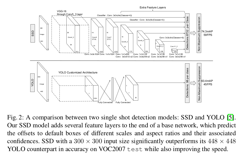
The details of the prior boxes are as follows:
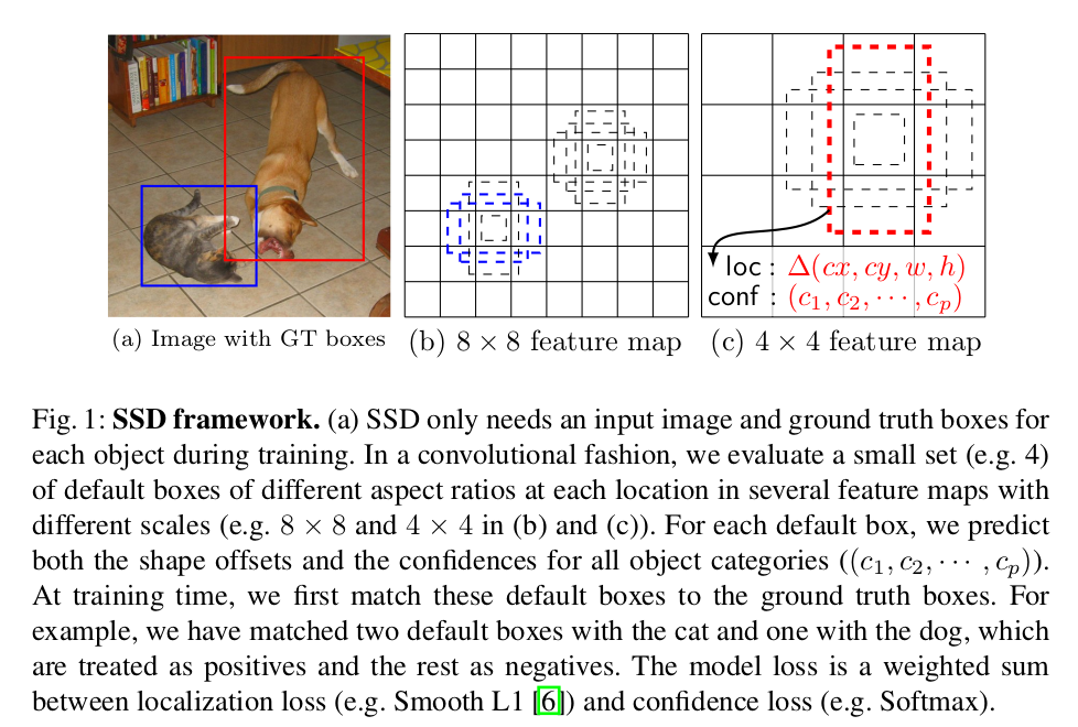
Model training
Training the $SSD$ model differs from training other typical detectors that use region proposals, mainly because $SSD$ needs to assign ground truth information to specific outputs in the fixed set of detector outputs (here are the authors’ own words: The key difference between training SSD and training a typical detector that uses region proposals, is that ground truth information needs to be assigned to specific outputs in the fixed set of detector outputs).
During training, $SSD$ needs to determine which prior box corresponds to which ground truth instance, and trains the model according to these mappings. According to the paper, the matching principle between prior boxes and $ground \ truth$ is as follows:
- For each $ground \ truth$ in the image, find the prior box with the largest $IoU$ with it, and that box matches it; this guarantees that every $ground \ truth$ matches some prior box;
- For the remaining unmatched prior boxes, if the $IoU$ with some $ground \ truth$ is greater than a preset threshold, then that prior box also matches this $ground \ truth$.
The matching principle above results in one $ground \ truth$ matching multiple prior boxes, but one prior box is not allowed to correspond to multiple $ground \ truth$.
The objective function for training $SSD$ comes from $MultiBox$, but the authors extended it to handle the multi-class classification problem. Define $x^P_{ij} \in \\{1,0\\}$ as an indicator function; $x^P_{ij}=1$ means that the $i$-th prior box matches the $j$-th $ground \ truth$ and the class of the $ground \ truth$ is $P$. Under the matching strategy above we can have $\sum_ix^P_{ij} \ge 1$. The overall loss function is the weighted sum of the localization loss and the confidence loss, as follows:
$$ L(x,c,l,g) = \frac{1}{N}(L_{conf}(x,c)+\alpha L_{loc}(x,l,g)) $$where $N$ denotes the number of positive samples among the prior boxes, $c$ is the predicted class confidence, $l$ is the predicted position of the bounding box corresponding to the prior box, and $g$ is the position parameter of the $ground \ truth$. The localization loss uses $Smooth \ L1 \ loss$; as in $Faster \ RCNN$, the authors regress the offsets of the prior box center $d(cx,cy)$ and of its width $w$ and height $h$. Note here that the ground truth $g$ must first be encoded, because the prediction $l$ is an encoded value.
$$ \begin{aligned} L_{loc}(x,l,g) & = \sum_{i\in Pos}^N \sum_{m\in \{cx,cy,w,h\}}x_{ij}^ksmooth_{L1}(l_i^m-\hat{g}_j^m) \\ \hat{g}_j^{cx} & = (g_j^{cx}-d_i^{cx})/d_i^w \\ \hat{g}_j^{cy} & = (g_j^{cy}-d_i^{cy})/d_i^h \\ \hat{g}_j^{w} & = log(\frac{g_j^w}{d_i^w}) \\ \hat{g}_j^{h} & = log(\frac{g_j^h}{d_i^h}) \\ \end{aligned} $$The confidence loss uses $softmax \ loss$.
$$ L_{conf}(x,c) = - \sum_{i \in Pos}^Nx_{ij}^Plog(\hat{c}_i^P)-\sum_{i \in Neg}log(\hat{c}_i^0) $$where
$$ \hat{c}_i^P = \frac{exp(c_i^P)}{\sum_Pexp(c_i^P)} $$To handle the problem of objects having different sizes, some methods suggest processing the image at different sizes and then merging the results; a similar effect can be obtained by making predictions from the feature maps of several different layers in a single network, and parameters can also be shared across all object scales. Previous experiments already verified that low-level feature maps produced by lower convolution layers can effectively improve semantic segmentation, because the lower network layers capture more detail of the input objects. In $SSD$ the authors use both low-level and high-level network layers for object detection.
Feature maps taken from different network layers have different sizes, and in the $SSD$ network the prior boxes do not need to correspond to the actual receptive field of each network layer; the authors designed the tiling of the prior boxes so that a particular feature map can respond to objects of a particular size. Suppose $m$ feature maps are used for prediction; the prior box size on each feature map is computed with the formula below:
$$ s_k = s_{min}+\frac{s_{max}-s_{min}}{m-1}(k-1), \ k \in [1,m] $$Here $s_{min}=0.2$ and $s_{max}=0.9$ are set, meaning the minimum size is 0.2 and the maximum size is 0.9. The scale of the prior boxes follows a linear increase rule: as the size of the feature map decreases, the scale of the prior boxes increases linearly. $s_k$ in the formula above denotes the ratio of the prior box to the image. The authors impose different aspect ratios on the prior boxes, denoted $a_r \in \\{1,2,3,\frac{1}{2},\frac{1}{3}\\}$, and compute the width and height of the prior boxes with the formulas below.
$$ \begin{aligned} w_k^a &= s_k\sqrt{a_r} \\ h_k^a &= s_k/\sqrt{a_r} \end{aligned} $$For the aspect ratio of 1, the authors add one more prior box (with scale $s_k^*=\sqrt{s_k s_{k+1}}$), so in the end each position of a feature map produces 6 prior boxes. The authors set the center coordinates of the prior boxes to $(\frac{i+0.5}{\vert f_k \vert},\frac{j+0.5}{\vert f_k \vert})$, where $\vert f_k \vert$ denotes the size of the k-th feature map and $i,j \in [0,\vert f_k \vert]$. In fact we can design the distribution of the prior boxes to suit a particular dataset. By combining the prior boxes generated from multiple feature maps of different sizes and aspect ratios the whole image can be fully covered, so $SSD$ can be regarded as dense sampling. Many of the generated prior boxes are negative samples, which shows that balancing positive and negative samples is necessary. The authors use hard negative mining for the balance: the prior boxes are sorted by their confidence loss, the top ones are picked, and the ratio of positive to negative samples is kept at $1:3$.
For data augmentation, the authors randomly choose one of the following for each training image:
- Use the original image in full;
- Sample a patch region so that the minimum $jaccard \ overlap$ with the objects is 0.1, 0.3, 0.5, 0.7 or 0.9;
- Randomly sample a patch region
where each patch region has a size $[0.1,1]$ times the original image size and an aspect ratio between 0.5 and 2. The $jaccard \ overlap$ (intersection over union, that is, IOU) is computed as follows:
$$ \begin{aligned} J(A,B) & = \frac{\vert A\cap B\vert}{\vert A\cup B\vert} \\ & = \frac{\vert A\cap B\vert}{\vert A \vert +\vert B\vert - \vert A\cap B\vert} \end{aligned} $$There is one point to note. In the $base \ network$, the authors use a $VGG16$ model pretrained on $ILSVRC \ CLS-LOC$, convert $fc6$ and $fc7$ into convolution layers, and change the pooling layer $pool5$ from the original $2\times 2$ with $stride=2$ to $3\times 3$ with $stride=1$. Here the authors use the $Atrous$ algorithm to let the model adapt to this change (in fact the $conv6$ layer uses dilated or atrous convolution to expand the receptive field without increasing the model parameters and complexity).
For more details of the model, refer to the original paper.
Appendix
While implementing this model, I was rather confused by the two parameters minsize and maxsize (these two parameters are used to generate the prior box size of each feature layer). After comparing with some other source codes, the rough computation process is as follows:
In theory, the computation should follow the formula given in the original paper:
$$ s_k = s_{min}+\frac{s_{max}-s_{min}}{m-1}(k-1), \ k \in [1.m] $$where $s_k$ is the ratio of the prior box size of each feature layer to the original image size, $S_{min}$ and $S_{max}$ denote the minimum and maximum ratio respectively — here $S_{min} = 0.2$ and $S_{max} = 0.9$ are set according to the paper — $m$ denotes the number of feature layers (after comparing several code bases, the m used is 5 rather than 6), and $k$ is the index of the feature layer.
In actual use, however, we need to take rounding into account, so the formula used is as follows (rounding up is used here, though other rounding methods can also be used):
$$ s_k = \lceil{s_{min} \times 100}\rceil+\left\lceil{\frac{\lceil{s_{max}\times 100}\rceil-\lceil{s_{min}\times 100}\rceil}{m-1}}\right\rceil(k-1), \ k \in [1,m] $$This gives a series of numbers:
$$ s1 \sim s6: 20, 38, 56, 74, 92, 110 $$Dividing them by 100 converts them into the real ratios:
$$ s1 \sim s6: 0.20, 0.38, 0.56, 0.74, 0.92, 1.10 $$Finally multiply by the original image size (300 is used here):
$$ 60, 114, 168, 222, 276, 330 $$For $s1$ there is also an $s1^{\prime}= 0.5\times s1$, and finally we get:
$$ 30, 60, 114, 168, 222, 276, 330 $$This gives 7 values, corresponding to 6 groups of $minsize$ and $maxsize$, from which the prior box size of each feature layer can be computed.
Reference
This post refers to:
Principle and implementation of SSD for object detection (author: Xiao Xiaojiang)