Object detection models come in single-stage and two-stage variants. Faster Rcnn is the representative of the two-stage kind; among single-stage models, besides SSD we also have another mainstream model, YoLo.
Introduction
Yolo turns the object detection problem into a regression problem over bounding boxes and class probabilities. It uses a single convolutional network to handle the prediction of multiple bounding boxes together with the class probabilities of those boxes, so the model runs very fast, though there is some loss in accuracy, since the candidate box generation process of something like Faster RCnn is gone. Secondly, the Yolo model has a lower background false positive rate and good generalization properties; the authors even ran object detection on abstract paintings, and the result was not bad :)
Design
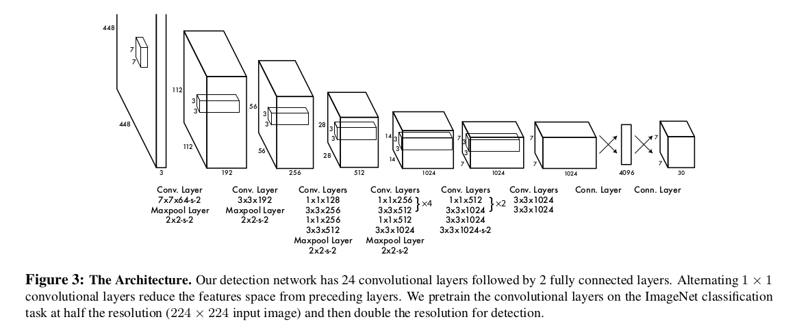
First the model divides the input image into $S \times S$ grids. If the center of an object falls inside a grid cell, that cell is responsible for predicting the object (specifically, during training the bounding box with the largest IOU with the ground truth box is selected to be responsible for detecting the corresponding ground truth instance. In this way each detector has its own job and only detects one class of object). Each grid cell predicts $B$ bounding boxes along with the confidence of these boxes. Here confidence means whether there is an object in the box and the confidence in that judgment: $Pr(Object)*IOU^{truth}_{pred}$. If there is no object in the box then $Pr(Object)$ is 0; otherwise the $IOU$ between the predicted box and the ground truth box is used as its confidence value.
Each bounding box contains 5 variables: $x,y,w,h,conf$. The first four are coordinate variables, where $x,y$ are the center of the box and $w,h$ denote the width and length. Note here that the center coordinates are relative to the grid cell size, while the width and height are relative to the whole image.
Each grid cell predicts $C$ class conditional probabilities ($C$ is the number of classes to predict). These probabilities are computed under the condition that an object is present: $Pr(Class_i\vert Object)$. During training, this probability is multiplied by the confidence of the box to obtain the predicted probability of each box for each class:
$$ Pr(Class_i\vert Object) * Pr(Object) * IOU^{truth}_{pred} = Pr(Class_i) * IOU^{truth}_{pred} $$In summary, the final output tensor of the model has size $S\times S\times (B*5+C)$. The authors chose the parameters $S=7$ and $B=2$, and the training dataset is $PASCAL \ VOC$, so the number of labels is $C=20$. A classic figure from the paper is included below:
Structure
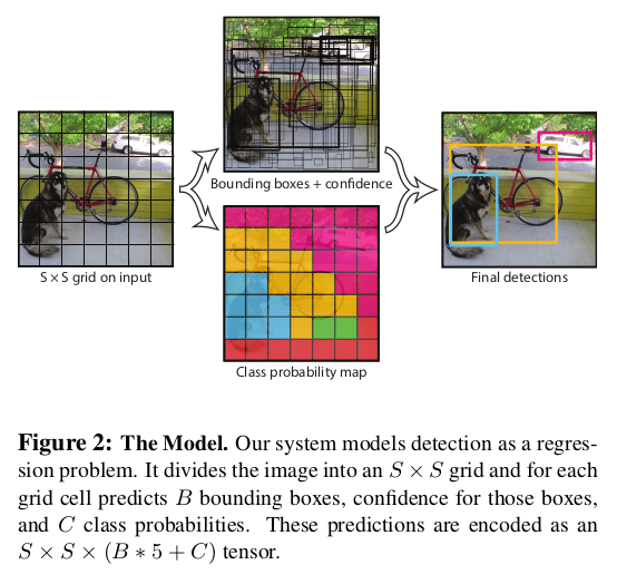
The overall model structure is a convolutional network to extract features plus fully connected layers to output the predicted probabilities and coordinate values. For the feature extraction part, the network built by the authors has a total of 24 convolution layers (for yolo tiny, 9 convolution layers are used along with a reduced number of kernels), and $1\times 1$ downsampling layers plus $3\times 3$ convolution layers are used to replace the inception part of GoogLeNet. The structure figure from the paper is attached as well:
Training
The authors use the Darknet framework for model training and inference. In the pretraining stage, the authors take the first 20 convolution layers of the model and attach a global average pooling layer and a fully connected layer to form a classification network, which is trained on the $ImageNet$ dataset. Since adding both convolution and connected layers to the pretrained model improves performance, the authors add four randomly initialized convolution layers (so the final model has 24 convolution layers) and two fully connected layers. Because object detection requires a higher resolution, the input images are raised from the pretraining size $224\times 224$ to $448\times 448$. The last layer predicts class probabilities and box coordinates simultaneously; here the box coordinates are normalized, as mentioned above (the center coordinates are relative to the grid cell size while the width and height are relative to the whole image). The activation function used in the network layers is $Leak\ ReLU$:
$$ \phi(x) = \begin{cases} x, \ &\text{if x > 0} \\ 0.1x, \ &\text{otherwise} \end{cases} $$The loss function chosen for the model is the sum-squared error loss function, because it is simple to optimize (yeah, sometimes you just overthink it); of course the authors made some adjustments to it to fit this model. Several shortcomings are listed here:
- The localization weight of some boxes that are not good enough is the same as the localization weight of boxes that are predicted well;
- Among the grid cells, there are sometimes many cells that contain no object, and the confidence of these cells is 0, so their gradients usually exceed the gradients of the boxes that contain objects, which makes the model unstable.
To compensate for these problems, the authors increase the coordinate loss of the bounding boxes through the parameter $\lambda_{coord}$ and decrease the confidence loss of boxes containing no object through $\lambda_{noobj}$; the paper sets $\lambda_{coord}=5$ and $\lambda_{noobj}=0.5$.
At the same time, the sum-squared error treats the error on large boxes and small boxes the same, which does not match our requirement that a small deviation in a large box should count for less than a small deviation in a small box. The authors take a clever approach: take the square root of the width and height of the box and then compute the squared error.
The final loss function is as follows:
$$ \begin{aligned} Loss =\ & \lambda_{coord}\sum_{i=0}^{S^2}\sum_{j=0}^B\mathbb{I}_{ij}^{obj}[(x_i-\hat{x}_i)^2+(y_i-\hat{y}_i)^2] \\ &+\lambda_{coord}\sum_{i=0}^{S^2}\sum_{j=0}^B\mathbb{I}_{ij}^{obj}\left[\left(\sqrt{w_i}-\sqrt{\hat{w}_i}\right)^2-\left(\sqrt{h_i}-\sqrt{\hat{h}_i}\right)^2\right] \\ &+\sum_{i=0}^{S^2}\sum_{j=0}^B\mathbb{I}_{ij}^{obj}(C_i-\hat{C}_i)^2 \\ &+\lambda_{noobj}\sum_{i=0}^{S^2}\sum_{j=0}^B\mathbb{I}_{ij}^{obj}(C_i-\hat{C}_i)^2 \\ &+\sum_{i=0}^{S^2}\mathbb{I}_i^{obj}\sum_{c \in classes}(p_i(c)-\hat{p}_i(c))^2 \end{aligned} $$Notes on the above:
$\mathbb{I}_i^{obj}$ is an indicator function indicating whether an object is present in the corresponding cell $i$;
$\mathbb{I}_{ij}^{obj}$ is also an indicator function, indicating whether the $j$th bounding box of cell $i$ is responsible for predicting an object.
The first two terms of the function are the coordinate prediction loss of the model, the third term is the confidence prediction loss of bounding boxes that contain objects, and the fourth term is the confidence prediction loss of bounding boxes that contain no object. The last term is the class loss of the model (note that this function only penalizes the classification loss of those cells that contain objects).
For the concrete parameter settings of training, refer to the original paper. To avoid overfitting, the authors also use Dropout layers and common data augmentation techniques.
Limitations
- Each cell only predicts 2 bounding boxes, and then each cell finally takes only the one with the highest IOU with the ground truth box as the final detection box, that is, each cell predicts at most one object, which is not good for detecting small objects;
- Although the loss function uses square roots to alleviate the problem that the same position error has the same effect on large and small boxes, the effect is small and does not fundamentally solve the problem;
- The model learns to predict bounding boxes from the data, so it is hard to generalize to objects with new or different aspect ratio configurations, and the model still uses fairly coarse features to generate bounding boxes.
Reference
This post is mainly based on the following paper: