After the yolov1 algorithm was released it caused a strong reaction among the public, and many researchers compared the algorithm with Fast Rcnn; yolov1 showed a fair number of deviations in object localization and had low recall. So in almost the same year the authors released yolov2, along with yolo9000 for detection over a huge number of classes — the iteration speed of this algorithm leaves one baffled (it really is awesome).
The authors mainly improve the algorithm model around a few points: raising the recall of the model and reducing object localization deviations while maintaining model accuracy, and they also propose a joint training method to realize the super-many-class detection algorithm yolo9000.
Better
The authors use many tricks to simplify the model while improving accuracy. The first is batch normalization, which can significantly improve the convergence of the model while requiring no other form of regularization, so layers such as the Dropout layer in yolov1 can be removed. The authors add a BN layer after every convolution layer, improving the model’s $mAP$ by at least $2\%$. When training the classification network, yolov1 used an input image resolution of $224\times 224$, while in actual detection the image resolution used is $448\times 448$; yolov2, by contrast, directly uses a size of $448\times 448$ when fine-tuning the classification network. This operation gives the model time to adapt to the change in resolution. After raising the resolution, the model’s $mAP$ improves by about $4\%$.
As is well known, yolov1 does not use the anchor boxes approach but predicts bounding boxes directly through fully connected layers; however, the authors found that predicting the box offsets is simpler than predicting the box coordinates and can simplify the network. So in yolov2 the fully connected layers are removed and anchor boxes are used to predict bounding boxes. Secondly, one pooling layer is removed so that the convolution layers of the network output a higher resolution, and an image input of $416\times 416$ is used instead of $448\times 448$. The reason for choosing $416\times 416$ here is that the authors want the final feature map to have an odd size (downsampling by 32 gives a final feature map of size $13\times 13$), so that there is a single center point on the feature map. An object, especially a large one, generally appears at the center of the image, so having a center point there to predict the bounding box works a bit better than the four surrounding points. After adopting the anchor boxes mechanism the $mAP$ of the model does not improve noticeably, and even drops slightly, but the recall does improve by a certain amount; in short, there is still room for improvement.
After introducing the anchor boxes mechanism, the authors face two problems:
- The size of the boxes. In the past the box sizes were chosen manually and then optimized by the network. Choosing good sizes improves the detection performance of the model enormously.
- The instability of the model. Most of the instability comes from the predicted bounding box coordinates $(x,y)$.
As for choosing the box sizes, the authors use the k-means clustering algorithm to select the anchor sizes (honestly, this move is slick). The goal of introducing anchor boxes is to give the detection boxes higher IOU values, but the usual K-means clustering algorithm uses the Euclidean distance formula, which does not meet the requirement, so the authors change the distance formula and use IOU to measure distance:
$$ d(box, centroid) = 1-IOU(box, centroid) $$Since a convolutional neural network is translation invariant and the positions of the anchor boxes are fixed by each grid cell, only the width and height of the anchors need to be computed by k-means. Through experiments, the authors finally choose k = 5.
As for the stability problem of the model, the authors follow yolov1’s approach, that is, predicting the offsets of the bounding box center relative to the top-left corner of the corresponding grid cell, and using a sigmoid function to constrain the box center within the current cell:
$$ \begin{aligned} b_x & = \sigma(t_x)+c_x \\ b_y & = \sigma(t_y)+c_y \\ b_w & = p_we^{t_w} \\ b_h & = p_he^{t_h} \\ Pr(object) * IOU(b, object) & = \sigma(t_o) \end{aligned} $$The explanation figure from the paper is attached:
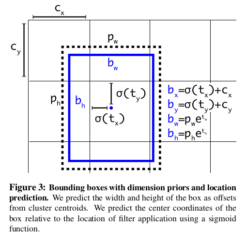
where $p_h$ and $p_w$ denote the sizes of the bounding boxes produced by k-means clustering
So the authors generate bounding boxes by using size clustering together with direct prediction of the box center position.
To let the model handle the detection of both large and small objects well, the authors introduce Fine-Grained Features. Instead of using only the last feature layer of $13\times 13$ to detect objects as yolov1 did, the model also adds information from the preceding feature layer ($26\times 26$), which gives rise to the passthrough layer. In the later code the authors borrow from ResNet and do not process the high-resolution image directly, but first apply a $1\times 1\times 64$ convolution. The logic of implementing the passthrough layer is roughly: take the lower-level feature map $26\times 26\times 512$, use $1\times 1\times 64$ to reduce the dimension to $26\times 26\times 64$, then split it into 4 parts and stack them along the channel dimension: $13\times 13\times 256$, which combined with the last layer’s $13\times 13\times 1024$ gives: $13\times 13\times (1024+256) = 13\times 13\times 1280$. This is roughly the processing of passthrough. After passing through the passthrough layer, the features are processed with $3\times 3$ and $1\times 1$ operations, and the output is $13\times 13\times 125$.
To make the model more robust, the authors also adopt multi-scale training. After training a certain number of batches, a size is randomly chosen from a size range as the input size of the training images (the paper changes it once every 10 batches). Because the model downsamples by 32, the input image size should be a multiple of 32, for example $\{320, 352, ..., 608\}$.
Faster
The feature extraction networks used by usual object detection models are based on VGG-16, a very powerful but somewhat bulky network. In the earlier yolov1 the authors used a feature extraction network based on the Googlenet architecture, which runs faster than VGG-16 but has lower accuracy than VGG-16. To improve both the efficiency and the performance of the model as much as possible, the authors redesigned yolov2.
And so Darknet-19 was born. This model is similar to VGG-16, mainly using $3\times 3$ convolution kernels and doubling the number of channels after each pooling operation. Following the conclusion of NIN (Network in Network), the authors use global average pooling while interleaving $1\times 1$ convolution kernels to compress the number of feature channels. BN layers are of course indispensable; BN layers not only accelerate model convergence but also regularize the model. In the end, Darknet-19 has 19 convolution layers and 5 max pooling layers; the concrete structure is shown below:
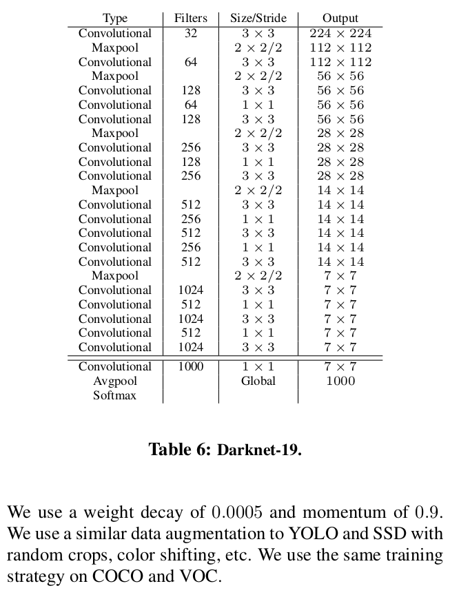
Once the feature extraction network is built, it is time to train it. The authors train it for $160$ iterations on the standard ImageNet 1000-class classification dataset with SGD, setting the initial learning rate to $0.1$. As for updating the learning rate, the authors use a polynomial decay strategy:
$$ lr_{cur} = (lr_{begin}-lr_{end})\cdot (1-\frac{gstep}{dstep})^{power} + lr_{end} $$where $lr_{begin}$ is the starting learning rate, $lr_{end}$ is the final learning rate, $dstep$ is the number of decay steps, $gstep$ is the number of global steps, and the following holds:
$$ gstep = \min(gstep, dstep) $$For the concrete parameter design, see the authors’ original paper.
After the initial training at a resolution of $224\times 224$, the input image resolution is raised to $448\times 448$ and the model is fine-tuned to adapt to large-resolution images.
After Darknet-19 training is finished, the authors remove its last convolution layer and add 3 convolution layers with $3\times 3\times 1024$ kernels, each followed by a $1\times 1$ convolution layer whose number of channels depends on the number of classes to detect. As for the passthrough layer mentioned earlier, the authors use it on the last $3\times 3\times 512$ layer and the second-to-last convolution layer.
That is the end of the YoLov2 part; what follows is where YoLo9000 takes the stage.
Stronger
To detect as many objects as possible, the authors propose a method for jointly training on classification datasets and detection datasets. During model training, the authors mix images from the two datasets; when a classification image is encountered, only the classification part of the network structure is used to backpropagate the loss, while when a detection image is encountered, backpropagation is based on the whole loss function. For mixing the datasets, one problem faced is how to unify the labels, and moreover the loss function used by most classification algorithms is the softmax function, which assumes that classes are mutually independent, which does not fit the logic here.
To address the problems above, the authors introduce hierarchical classification, similar to the species tree in biology. Here WordNet is used (the labels of the Imagenet dataset are taken from it); it is a cognition-based language database structured as a directed graph. The authors do not use the whole graph structure (after all, the graph is enormous) but build the graph structure using only the concepts in Imagenet. To build the graph, the paths of the various Imagenet labels to the root node in WordNet are compared: words with a unique path are added to the graph, and for those with multiple paths to the root node the shortest path is chosen and added to the graph, finally producing a $WordTree$.
Given a synset, the conditional probability of each node is predicted, for each hyponym of that synset. For example, at the terrier node the model predicts:
$$ Pr(Norfolk\ terrier\vert terrier) \\ Pr(Yorkshire\ terrier\vert terrier) \\ Pr(Bedlington\ terrier\vert terrier) \\ ... $$To compute the absolute probability of a particular node, one simply follows the path from that node to the root of the tree and multiplies the conditional probabilities of the nodes along the path. For example, for the Norfolk terrier node:
$$ Pr(Norfolk\ terrier) = Pr(Norfolk\ terrier\vert terrier) \
- Pr(terrier\vert hunting\ dog) \
- … \ * \
- Pr(mammal\vert animal) \
- Pr(animal\vert physical\ object) $$
Here, for classification purposes, $Pr(physical\ object) = 1$ is assumed, that is, the image always contains an object.
A WordTree is built on top of the 1000 Imagenet classes to train Darknet-19; after adding all intermediate nodes, the number of labels expands from 1000 to 1369. During training, ground truth labels are propagated upwards, for example a label of “Norfolk terrir” should also be labeled “dog” and “mammal”. To compute the conditional probabilities, the model predicts a vector of length 1369 and computes the softmax over all synsets sharing the same concept, as shown below:
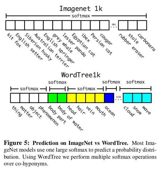
At classification time, the authors assume that each image contains one object; for the detection task, the value of $Pr(physical\ object)$ is no longer fixed at 1 but is given by the object detector of Yolov2. The detection part of the model gives a bounding box for the object along with its probability, and then traverses down the WordTree to find the highest-confidence path for each softmax branch until a certain threshold is reached; the node farthest from the root along that path is then the predicted label.
When merging the Imagenet dataset and the COCO dataset, because the sizes of the two datasets differ greatly, the authors resample the COCO dataset, so the final ratio of the two datasets is roughly $4:1$. The model keeps the YoLov2 structure but is changed to use 3 anchors (instead of 5) to limit the output size. During classification, the model backpropagates only the classification loss part, and backpropagates the objectness loss when the IOU between the predicted box and the ground truth label box is at least 0.3; during detection, the model backpropagates normally.
For the concrete details, refer to the original paper
Reference
This post refers to the following: