Yes, it has arrived.
Introduction
With a $320\times 320$ resolution input, yolo3 keeps its accuracy at $28.2mAP$ and runs in roughly $22ms$.
Compared with yolo2, this model does not bring any major changes; the authors tried many tricks to improve model performance, and finally selected the ones that proved useful and combined them into yolo3.
Bounding box and class prediction
In yolo2, bounding boxes are obtained by predicting the center coordinates of the box relative to the top-left corner of the image and the width and height relative to the anchors:
$$ \begin{aligned} b_x & = \sigma(t_x)+c_x \\ b_y & = \sigma(t_y)+c_y \\ b_w & = p_we^{t_w} \\ b_h & = p_he^{t_h} \\ \end{aligned} $$The bounding box prediction method of yolo2 is carried over here. yolo3 uses logistic regression to score the objectness of each anchor. When an anchor covers a ground-truth object over a larger area than any other box, that box is assigned a score of 1; when a box is not the best bounding box but does overlap some ground-truth object by more than a threshold (the authors chose 0.5 in the paper), the authors still ignore it. So the authors assign exactly one anchor to each ground-truth object; for the anchors that are not assigned, no coordinate or class loss is incurred, only the objectness loss. This way unnecessary boxes are removed and computation is reduced.
As for class prediction, yolo3 uses multi-label classification for each box to predict the classes the box may contain. The authors do not use softmax here because they found it has no impact on the high performance of the model, and an independent logistic classifier with a binary cross-entropy loss makes it easy to transfer the model to other datasets.
Model improvements
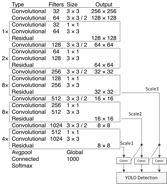
For training, the authors combine features across scales for prediction. yolo3 uses 3 different aspect ratios to predict boxes, in a way similar to the $FPN$ feature pyramid. The authors add several convolution layers after the feature extractor of the model to obtain a 3D tensor (containing bounding boxes, objectness probabilities and per-class probabilities). Then they take the feature map from two layers back, upsample it and concatenate it with the output of the last layer, which gives meaningful semantic information from earlier layers as well as fine-grained detail. The same procedure is repeated for one more merged layer, so the final model predicts at 3 different scales. For the choice of anchors, the authors follow yolo2 and use $k-means$ clustering to obtain candidate box sizes. Unlike yolo2, the authors choose 9 sizes and distribute them evenly among 3 different aspect ratios. The structure is shown below:
Feature extractor
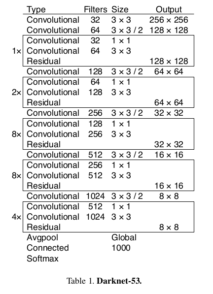
In yolo3 the authors use a brand-new feature extractor. The new convolution stack uses consecutive $3\times 3$ and $1\times 1$ kernels and adds residual blocks. The whole feature extractor has 53 layers, hence it is called $Darknet-53$. The structure is shown below:
Training and shortcomings
yolo3 is still trained on datasets without hard negative mining, while using multi-scale training, a large number of data augmentation methods, batch normalization and so on. On the new evaluation method of the COCO dataset, the mAP of the model is on par with the SSD model, but SSD runs about 3 times faster than yolo3. Under the old evaluation method, on the other hand, the mAP of the model is comparable to RetinaNet and leaves SSD far behind.
yolo3 still has some shortcomings. In earlier versions, yolo had always performed poorly on small object detection; after multi-scale training the model improved a lot on small objects, but its performance on medium and large objects is worse than before.
Reference
This post is mainly based on the following: