Papers keep piling up before I know it, and it is quite exhausting. Back to the point: neural networks are already applied in many fields and even surpass human ability in image recognition, but the improvement in model accuracy comes at the cost of higher computing requirements. Real engineering applications often cannot provide much computing power, and some algorithms have to run on embedded platforms, which means those fancy algorithms simply cannot be deployed. Following mobilenetv1, Google proposed its improved version mobilenetv2, which is better suited to lightweight deployment and can keep a decent accuracy while maintaining running speed.
Depthwise separable convolution
First let us look at the depthwise separable convolution already used in mobilenetv1. The general idea is to split an ordinary convolution into two steps: a depthwise convolution and a pointwise convolution, which reduces the amount of computation while achieving the same effect.
Suppose the input of a standard convolution is $L_i$ of dimension $h_i\times w_i\times d_i$, the kernel parameter is $K\in R^{k\times k\times d_i\times d_j}$, and the final output is $L_j$ of dimension $h_i\times w_i\times d_j$. So the computational cost of the standard convolution is $h_i\times w_i\times k\times k\times d_i\times d_j$.
With a depthwise separable convolution, the input is $L_i$ of dimension $h_i\times w_i\times d_i$, the depthwise convolution kernel parameter is $K_1\in R^{k\times k\times d_i\times d_i}$, the pointwise convolution kernel parameter is $K_2\in R^{1\times 1\times d_i\times d_j}$, and the final output is again $L_j$ of dimension $h_i\times w_i\times d_j$. So the computational cost is $k\times k\times h_i\times w_i\times d_i + 1\times 1\times h_i\times w_i\times d_i\times d_j$, that is $h_i\times w_i\times d_i\times (k^2 + d_j)$. It differs from the standard convolution by a factor of $\frac{k^2d_j}{k^2+d_j}$, so the depthwise separable convolution really is an efficient convolution design.
In the paper, mobilenetv2 uses $3\times 3$ kernel parameters throughout the separable convolutions.
Linear Bottlenecks
Let us just call it the linear bottleneck layer (I don’t know a good translation…). This part is mainly about the feature preservation ability of the model. It has long been believed that the “manifold of interest” in neural networks (presumably meaning something like the effective features) can be embedded in a low-dimensional subspace, hence the idea of reducing the dimension of convolution layers to reduce the dimension of the subspace and thereby obtain more effective features. However, this intuition breaks down when we recall that deep convolutional neural networks actually have non-linear per coordinate transformations.
Taking the ReLU activation function as an example: applied to a straight line in 1D space, it produces rays in n-dimensional space, and in general produces a piecewise linear curve with n joints. From the shape of the ReLU curve we can also see that a deep network only has a linear classifier function in the non-zero part of the output domain. The authors finally give two requirements for the main features of the model to lie in a low-dimensional subspace of a high-dimensional space:
- When the ReLU output is non-zero, ReLU is just a simple linear transformation;
- Provided that the input manifold lies in a low-dimensional subspace of the input space, ReLU can preserve the information of the input manifold
Assuming the second point holds, we can capture effective features by inserting linear bottleneck layers into the convolution block. The authors also show experimentally that adding linear bottleneck layers effectively prevents the nonlinear transformation from destroying too much feature information.
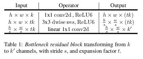
An important parameter in the linear bottleneck layer is the expansion ratio, that is, the ratio between the size of the input bottleneck and the internal size.
I am still a bit confused by this part, so I need to read it a few more times.
Inverted residuals
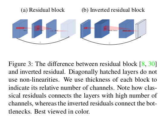
Inspired by the bottleneck idea, the bottleneck actually contains all the necessary information while the expansion layer merely acts as an implementation detail of the tensor’s nonlinear transformation, so the authors use shortcut connections directly between bottlenecks. This is shown below.
The rough structure of the bottleneck is shown below:
Model structure
As shown
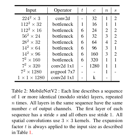
It starts with a standard convolution layer with 32 kernels, followed by 19 residual bottleneck modules (although the table in the paper only lists 17, and the official implementation also follows the table). The activation function is ReLU6 and the kernel size is $3\times 3$. Except for the first bottleneck, the authors use a constant expansion rate throughout the network (experiments show that model robustness is better when it is between 5 and 10)
The model implementation also contains some memory-efficiency improvements; see the original paper for details.
Finally, for the object detection field, the authors also modified the SSD network and proposed a lightweight implementation called SSDLite. On top of mobilenetv2, the first layer of SSDLite is connected to the expansion of layer 15 of mobilenetv2 (output stride 16), and the remaining SSDLite layers are attached on top of the last layer (output stride 32).
Reference
This post is mainly based on the following paper