IoU is an important metric in object detection; it measures how good a predicted box is by computing the ratio of the intersection to the union of the predicted box and the ground truth box. But the usual bounding box adjustment function generally adopts the L2 norm, that is, the loss is computed in an MSE manner, and some studies have shown that this is not the optimal optimization function, hence the IOU loss functions.
Computation of IoU:
$$ IoU = \frac{\vert B \cap B^{gt}\vert}{\vert B \cup B^{gt}\vert} $$where $B$ denotes the predicted box and $B^{gt}$ denotes the ground truth box; overall $IoU$ is the ratio of the intersection of the predicted and ground truth boxes to their union. It can effectively reflect the detection quality of the predicted box, and it is also scale invariant, that is, insensitive to scale.
IoU Loss
From the $IoU$ formula we can obtain a loss function simply and crudely:
$$ \mathcal{L}_{IoU} = 1-IoU = 1-\frac{\vert B \cap B^{gt}\vert}{\vert B \cup B^{gt}\vert} $$This loss function has an unavoidable flaw: when the two boxes do not intersect, the loss is constantly 1, so a non-intersecting box that is close and one that is far away give the same output; the direction of the gradient is lost and optimization is impossible.
Note: $Iou \ Loss$ has more than the implementation mentioned above; for example, there is the cross-entropy form of $UnitBox$ and the $Smooth-L1$ form of $IoUNet$, but they all share the problem above.
GIoU Loss (generalized IoU loss)
To solve the problem above, $GIoU$ appeared. It adds a penalty term on top of $IoU \ loss$. The larger the distance between the predicted box and the ground truth box, the larger the value of the penalty term. The concrete formula is as follows:
$$ \mathcal{L}_{GIoU} = 1-IoU+\frac{\vert C-B\cup B^{gt}\vert}{\vert C\vert} $$where $C$ is the smallest enclosing box containing both the predicted box and the ground truth box. During training, $GIoU \ loss$ tends to first enlarge the predicted box so that it overlaps the ground truth box, and then, guided by the $IoU$ term in the formula, maximizes the overlapping region. But when the ground truth box completely contains the predicted box, the penalty term in the formula above becomes 0, that is, $GIoU loss$ degrades to $IoU \ loss$, and because this loss relies too heavily on the $IoU$ term, more iterations are needed to converge, especially in the horizontal and vertical directions.
DIoU Loss (Distance-IoU loss)
Just like $GIoU$, $DIoU$ also adds a penalty term on top of $IoU \ loss$, but $DIou$ takes into account the distance between the predicted and ground truth boxes, the overlap ratio and the scale, specifically as follows:
$$ \begin{aligned} \mathcal{L}_{DIoU} & = 1-IoU+\mathcal{R}(\mathcal{B}, \mathcal{B}^{gt}) \\ \mathcal{R}_{DIoU} & = \frac{\rho^2(b, b^{gt})}{c^2} \end{aligned} $$where $b$ and $b^{gt}$ denote the center points of the predicted box and the ground truth box respectively, $\rho$ is the distance formula between the two points — here the Euclidean distance between the two center points — and $c$ is the diagonal distance of the smallest box containing the predicted box and the ground truth box, as shown in detail below.
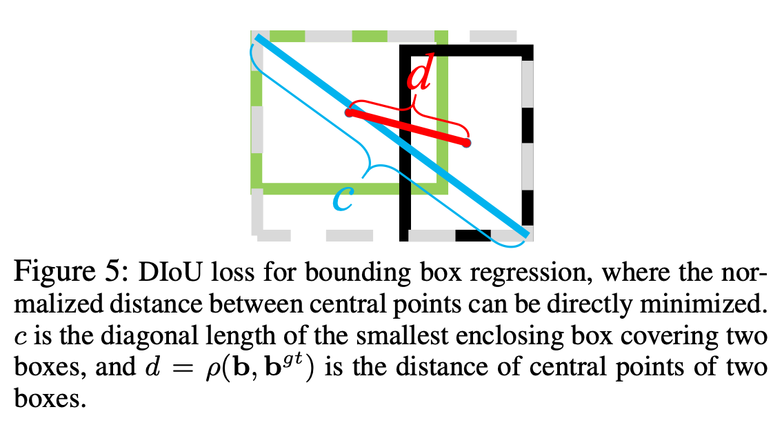
This loss function directly minimizes the distance between the two boxes, so it converges faster than $GIoU$. $DIoU$ can also be applied to $NMS$, making the resulting boxes more reasonable.
CIoU (Complete IoU Loss)
Taking the aspect ratio of the boxes into account on top of $DIoU$ gives $CIoU$, specifically as follows:
$$ \begin{aligned} \mathcal{L}_{CIoU} & = 1-IoU+\mathcal{R}(\mathcal{B}, \mathcal{B}^{gt}) \\ \mathcal{R}_{CIoU} & = \frac{\rho^2(b, b^{gt})}{c^2}+\alpha \mathcal{v} \\ \mathcal{v} & = \frac{4}{\pi^2}\left(arctan\frac{\mathcal{w}^{gt}}{\mathcal{h}^{gt}}-arctan\frac{\mathcal{w}}{\mathcal{h}}\right)^2 \\ \alpha & = \frac{\mathcal{v}}{(1-IoU)+\mathcal{v}} \end{aligned} $$Note:
The gradient of $CIoU$ contains the gradient of $\mathcal{v}$, which is roughly as follows:
$$ \begin{aligned} \frac{\partial\mathcal{v}}{\partial\mathcal{w}} & = \frac{8}{\pi^2}\left(arctan\frac{\mathcal{w}^{gt}}{\mathcal{h}^{gt}}-arctan\frac{\mathcal{w}}{\mathcal{h}}\right)\times\frac{\mathcal{h}}{\mathcal{w}^2+\mathcal{h}^2} \\ \frac{\partial\mathcal{v}}{\partial\mathcal{h}} & = -\frac{8}{\pi^2}\left(arctan\frac{\mathcal{w}^{gt}}{\mathcal{h}^{gt}}-arctan\frac{\mathcal{w}}{\mathcal{h}}\right)\times\frac{w}{\mathcal{w}^2+\mathcal{h}^2} \end{aligned} $$When the aspect ratio is in $[0,1]$, the value of $\mathcal{w}^2+\mathcal{h}^2$ is usually very small, so $\frac{1}{\mathcal{w}^2+\mathcal{h}^2}$ becomes rather large and may cause gradient explosion; therefore in implementations it is usually replaced by the constant 1.
Reference
This post refers to the following:
Distance-IoU Loss: Faster and Better Learning for Bounding Box Regression