At the end of 2019 and the beginning of 2020, Google Brain published two papers proposing a fast and accurate model for image classification and for object detection respectively, naming them EfficientNet and EfficientDet. The authors also adjusted the model parameters to obtain a series of efficient classification and detection models.
EfficientNet
From previous work and their own experiments, the authors summarized two observations:
- Scaling any single dimension of a model (depth, width, resolution) improves the model’s accuracy, but for very large scaling factors the accuracy gain diminishes
- In scaling a convolutional network, scaling all dimensions of the model in a balanced way yields better accuracy and speed
compound scaling
Based on the two observations above, the authors no longer use the traditional single-dimension model scaling but scale all dimensions of the model (depth, width and resolution).
First, for a convolution model we can write:
$$ \mathcal{N} = \underset{i=1...s}{\bigodot}\mathcal{F}_i^{L_i}(X_{\langle H_i, W_i, C_i\rangle}) $$where $\mathcal{F}_i^{L_i}$ means that in network block $i$ the network layer $F_i$ is repeated $L_i$ times, $\langle H_i,W_i,C_i\rangle$ denotes the input size of the $i$-th layer, and $\mathcal{N}$ is the whole convolutional network model.
From the formula above we get the abstracted model scaling optimization problem:
$$ \begin{aligned} \underset{d,w,r}{max} &\ Accuracy(\mathcal{N}(d,w,r)) \\ s.t. &\ \mathcal{N} = \underset{i=1...s}{\bigodot}\hat{\mathcal{F}}_i^{d\cdot \hat{L}_i}(X_{\langle r\cdot \hat{H}_i, r\cdot \hat{W}_i, w\cdot \hat{C}_i\rangle}) \\ &\ \text{Memory}(\mathcal{N}) \le target\_memory \\ &\ \text{FLOPS}(\mathcal{N}) \le target\_flops \end{aligned} \tag{1} $$where $L_i,H_i,W_i,C_i$ denote the model depth, input length, input width and model width after scaling respectively. $w,d,r$ are the scaling coefficients corresponding to the model width, depth and resolution.
The authors use a scaling ratio coefficient $\phi$ to uniformly scale all dimensions of the model:
$$ \begin{aligned} \text{depth:} & \ d = \alpha^\phi \\ \text{width:} & \ w = \beta^\phi \\ \text{resolution:} & \ r = \gamma^\phi \\ s.t. & \ \alpha \cdot \beta^2 \cdot \gamma^2 \approx 2 \\ & \ \alpha \ge 1,\beta \ge 1,\gamma \ge 1 \\ \end{aligned} \tag{2} $$where $\alpha,\beta,\gamma$ are constants that can be determined by a small grid search. As for the constraint $\alpha\cdot\beta^2\cdot\gamma^2\approx 2$ given by the authors, it means that the scaled model will have roughly $2^\phi$ times the floating point operations of the original model, because doubling the model depth doubles the model’s computation, while doubling the model width or resolution increases the computation fourfold, so the base factor by which the model’s computation grows is $\alpha\cdot\beta^2\cdot\gamma^2$.
Architecture
To get better results, the model baseline is also a very important component; the authors used network search to find the EfficientNet-B0 network within a constrained search space. The search targets $ACC(m)\times[FLOPS(m)/T]^w$, where $ACC(m)$ denotes the model accuracy, $FLOPS(m)$ denotes the model’s computation, $T$ is the computation target of the model and $w=-0.07$ is a hyperparameter controlling the balance between accuracy and computation; the reason for using computation rather than inference latency as the evaluation target is that the authors want to decouple the model from the device, since the inference latency differs across devices while the computation is the same. The final model baseline is as follows:
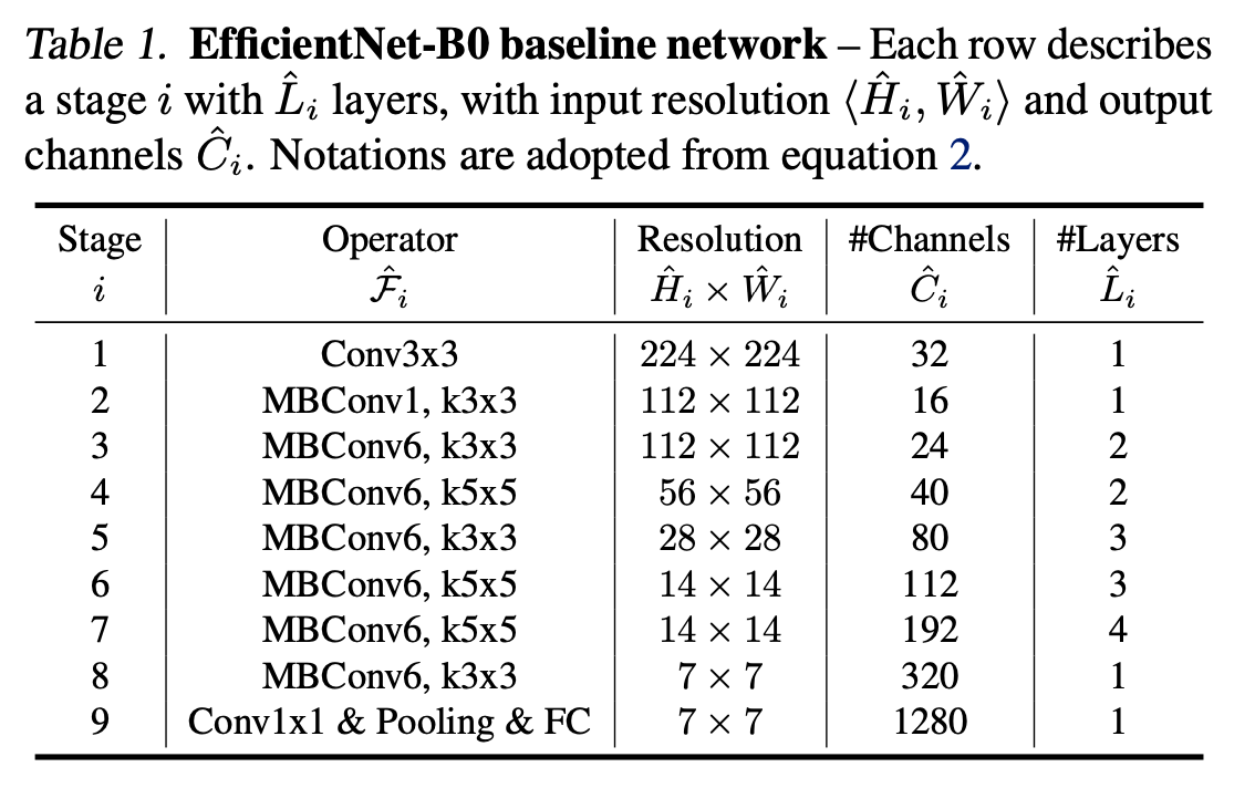
From the figure we can see that its main components are MBConv and the SE block. MBConv is the inverted bottleneck used in Mobilenetv2, while the SE block is similar to an attention mechanism — a lightweight module that optimizes the model.
Starting from the resulting baseline, the following two scaling steps give the final series of classification models:
- First fix $\phi=1$ and, assuming more available resources, perform a small grid search over $\alpha,\beta,\gamma$ based on equations 1 and 2. The best values under the constraint $\alpha\cdot\beta^2\cdot\gamma^2\approx 2$ turn out to be $\alpha=1.2,\beta=1.1,\gamma=1.15$, which are used as the parameters of the EfficientNet-B0 model.
- Fix $\alpha,\beta,\gamma$ and scale with different $\phi$ using equation 3 to obtain the B1 to B7 models.
At this point the eight models EfficientNet-B0 to B7 have been constructed.
EfficientDet
To obtain an accurate and fast object detection model, the authors propose the EfficientDet model based on a single-stage detection algorithm, mainly solving the following two problems:
- How to perform efficient multi-scale feature fusion — the authors’ answer is BiFPN
- How to scale the model effectively — here the authors apply the same compound scaling method as in EfficientNet
BiFPN
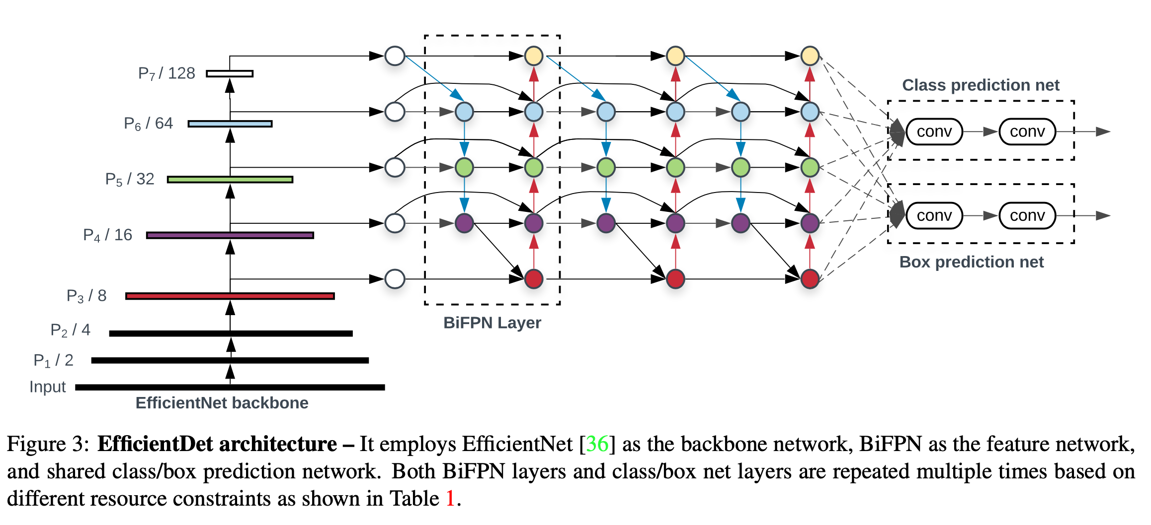
The purpose of multi-scale feature fusion is to aggregate features from different resolutions so that the model generalizes better. FPN is an effective means of multi-scale feature processing; it adds a top-down path to obtain information from other branches. But since there is only one path, its expressive power is limited, so PANet was later proposed, adding a bottom-up path on top of FPN. After that, researchers used network search to find NAS-FPN, whose expressive power is higher than PANet, but its computation is enormous and it is not suitable for practical scenarios. Finally the authors propose BiFPN, whose structure is as follows:

BiFPN is improved on top of PANet. First, the authors remove the nodes in PANet that have only a single input, in order to simplify the model, because nodes with only a single input do not need feature fusion and contribute relatively little in a structure whose purpose is feature fusion, so removing them has little impact. Second, an extra connection is added between the input and output nodes of the structure, so as to fuse more features without adding too much computation. Finally, unlike PANet which has only one top-down and one bottom-up path, the authors reuse BiFPN repeatedly to allow the fusion of the high-level features extracted by the model.
When fusing features, the usual approach is to unify the size of each feature map and then add them up, which means feature maps of different resolutions have the same weight when fused, with no difference. However, the authors observe that different resolutions contribute differently to the final output of the model, so treating feature inputs of different resolutions with equal importance is inappropriate. Based on this idea, the authors consider three weighting methods:
- Unbounded fusion: $O = \sum_i w_i\cdot I_i$, where $w_i$ is a learnable network weight, which can be a scalar (weighting each feature), a vector (weighting each channel) or a tensor (weighting each pixel). Using scalars for weighting gives a considerable accuracy gain with minimal computation, but scalar weights can be very large or very small, which makes model training unstable. For this reason the authors adopt weight normalization to bound the range of each weight.
- Softmax-based fusion: $O = \sum_i\frac{e^{w_i}}{\sum_je^{w_j}}\cdot I_i$, that is, using softmax for weighting, so the range of the weights is fixed between 0 and 1, and the values represent their respective importance. But the extra softmax computation is rather slow; to reduce the cost the authors propose the weighting method below.
- Fast normalized fusion: $O = \sum_i\frac{w_i}{\epsilon+\sum_jw_j}\cdot I_i$, where $w_i \ge 0$ is guaranteed by applying the activation function $Relu$ beforehand. This method avoids the time-consuming softmax operation.
Finally, BiFPN consists of bidirectional cross-scale connections and weighted feature fusion as shown in the figure above. To speed things up, the authors also replace the convolutions in the feature fusion part with separable convolutions, and add batch normalization to BiFPN with an activation function computed after every convolution.
Note: Note here that the input nodes used for the input-to-output connections of BiFPN and for the input-to-intermediate-node connections are different nodes with the same values. For details see this article.
The rough structure of EfficientDet is finally as follows:
compound scaling
Compound scaling uses a method similar to EfficientNet, except that for object detection models there are more dimensions to scale; here the authors use a heuristic-based scaling method, again with $\phi$ as the scaling coefficient.
For the backbone, the authors use the EfficientNet-B0 to B6 models.
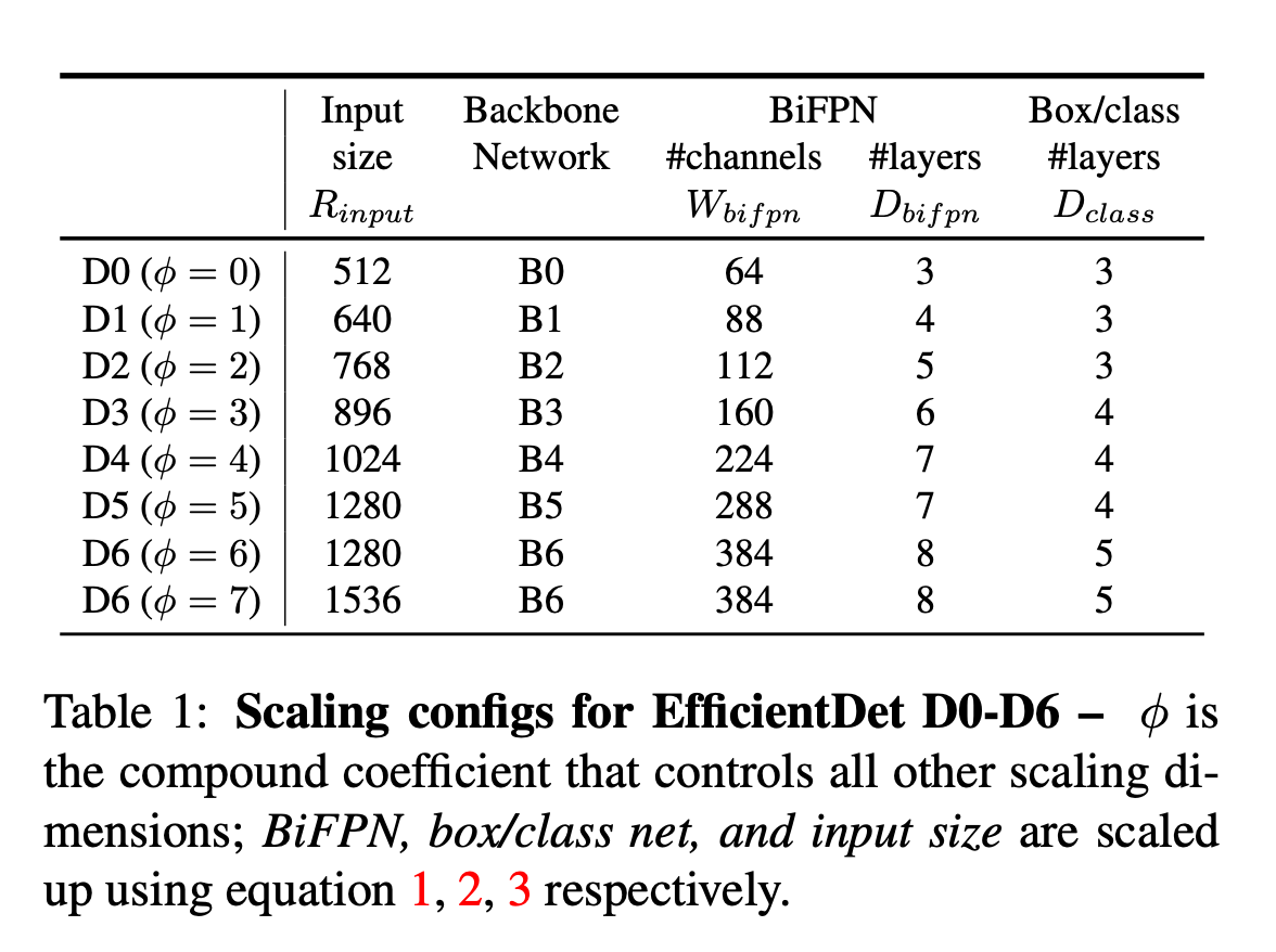
BiFPN scaling. The BiFPN depth $D_{bifpn}$ is increased linearly, while the BiFPN width $W_{bifpn}$ is increased exponentially. The authors then performed a grid search over ${1.2,1.25,1.3,1.35,1.4,1.45}$ to obtain the best scaling base of $1.35$, and finally scale as follows:
$$ \begin{aligned} W_{bifpn} & = 64 \cdot 1.35^\phi \\ D_{bifpn} & = 3 + \phi \end{aligned} $$For the prediction head, its width is fixed to the width of BiFPN, that is, $W_{pred}=W_{bifpn}$, but its depth is increased linearly:
$$ D_{box} = D_{class} = 3+\lfloor \phi/3\rfloor $$As for the input image resolution, because feature levels 3 to 7 of the model are used by BiFPN, the input dimension must be a multiple of $2^7=128$. It is increased linearly as follows:
$$ R_{input} = 512+\phi\cdot 128 $$Through this series of operations we obtain eight object detection models, EfficientDet-D0 to D7; EfficientDet-D6 and D7 have the same parameters except for the resolution parameter. Specifically:
Reference
This post is mainly based on the following articles:
EfficientNet: Rethinking Model Scaling for Convolutional Neural Networks
The unglamorous pytorch implementation of efficientdet that topped the SoTA charts