Usual object detection algorithms are all based on Anchors; although this generates many useless anchor boxes and brings a time-consuming NMS post-processing step, the accuracy of the algorithm is higher, because the anchor boxes basically cover all object regions. There is another approach in the detection field based on Anchor free, that is, without anchor boxes; as far as I know these are mainly Cornernet, Centernet (Keypoint Triplets for Object Detection) and Centernet (Objects as Points). This type of algorithm does not need to generate anchor boxes, and therefore does not need the time-consuming NMS post-processing. Here I mainly record the processing method of Centernet (Objects as Points).
Model structure
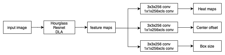
Centernet mainly borrows the operation of keypoint detection to detect the center position of an object, and extends it to the object detection field, that is, obtaining the box size through regression. This algorithm can be conveniently extended to other fields, such as the object detection, 3D box prediction and pose mentioned in the paper. For the backbone the authors mainly use hourglass, resnet and DLA models; for object detection, three branches are added after the backbone, mainly: a Heat maps branch to obtain the object center point, Center offset to correct the object center point, and Box size to regress the object box size. The rough structure is as follows (where cls denotes the number of classes to detect):
Data flow
Having described the model structure, next comes the data processing. The authors annotate the object center points with a heat map, and the heat map is produced by a Gaussian kernel.
First the $H\times W\times 3$ image is downsampled (the downsampling factor $R$ is set to $4$ here) to give an image of $H/R\times W/R\times cls$, where $cls$ is the number of classes. Then the center point of the ground truth box on the scaled image is computed: $\hat{p}(x,y)=\lfloor\frac{p}{R}\rfloor$, and the center point is mapped through the Gaussian kernel $exp(-\frac{(x-\hat{p}_x)^2+(y-\hat{p}_y)^2}{2\sigma_p^2})$, finally giving the heat map $\hat{Y}\in [0,1]^{\frac{W}{R}\times\frac{H}{R}\times 3}$.
The generated heat map does not have 1 at the center point position and 0 elsewhere. It is 1 at the object point and gradually decreases as it spreads outward. In the Gaussian kernel mapping, the corresponding Gaussian function is drawn centered at $\hat{p}$ and the region with $\hat{p}$ as the center and $radius$ as the radius is cropped out; meanwhile $\sigma_p$ in the Gaussian kernel is the standard deviation adapted to the object size, which in the authors’ implementation is set to $\frac{2\times radius}{6}$. The design of the cropped region radius $radius$ and of the Gaussian kernel parameter $\sigma_p$ here both refer to another paper, Cornernet. In Cornernet, the standard deviation of the Gaussian kernel is designed to be $\frac{1}{3}$ of the radius of the allowed deviation region (that is, $radius$). Considering that a box generated by a point near the object point (the object point in Cornernet being the corner of the object box) will have a fairly large IoU with the object box, directly assigning 0 to that point is inappropriate, so an allowed deviation region is formed by setting an IoU threshold (set to 0.7 in Centernet), within which the values of the points around the object point gradually decrease following the Gaussian function. The boxes generated by these points have three limiting cases of intersection with the object box; the region radius is computed for each of the three cases, and the smallest of the three radii is taken as the value of $radius$.
Computing radius
The generated box circumscribes the object box
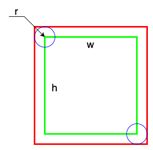
From the figure above the IoU can be computed:
$$ IoU = \frac{w\cdot h}{(w+2r)\cdot(h+2r)} \ge iou\_overlap $$so the maximum radius in this case satisfies:
$$ \begin{aligned} & \frac{w\cdot h}{(w+2r)\cdot(h+2r)} = k = iou\_overlap \\ \Rightarrow & \ 4k\cdot r^2 + 2k(w+h)\cdot r + (k-1)wh = 0 \end{aligned} $$This is a quadratic equation in one variable; provided it has a solution, the positive solution for $r$ can be computed with the formula. ($y = \frac{-b\pm\sqrt{b^2-4ac}}{2a}$, where $b^2-4ac\ge 0$).
The generated box is inscribed in the object box
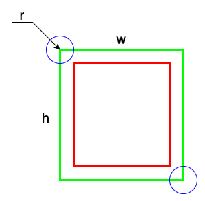
From the figure above the IoU can be computed:
$$ IoU = \frac{(w-2r)\cdot(h-2r)}{w\cdot h} \ge iou\_overlap $$so the maximum radius in this case satisfies:
$$ \begin{aligned} & \frac{(w-2r)\cdot(h-2r)}{w\cdot h} = k =iou\_overlap \\ \Rightarrow & \ 4\cdot r^2 - 2(w+h)\cdot h + (1-k)wh = 0 \end{aligned} $$The positive solution for $r$ can likewise be obtained
The generated box is half circumscribed and half inscribed with respect to the object box
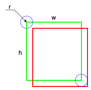
The IoU can be computed as follows:
$$ IoU = \frac{(w-r)\cdot(h-r)}{2\cdot h\cdot w - (w-r)\cdot(h-r)} \ge iou\_overlap $$so the maximum radius in this case satisfies:
$$ \begin{aligned} & \frac{(w-r)\cdot(h-r)}{2\cdot h\cdot w - (w-r)\cdot(h-r)} = k = iou\_overlap \\ \Rightarrow & \ (1+k)\cdot r^2 - (w+h)(1+k)\cdot r + (1-k)wh = 0 \\ \Rightarrow & \ r^2 -(w+h)\cdot r + \frac{1-k}{1+k}wh = 0 \end{aligned} $$Similarly the positive solution for $r$ can be found
Taking all three cases together, the smallest of the three is taken as the value of $radius$.
Loss function
This model has good scalability; by adding different branches it can be applied to different fields, among which two branches are fixed (Heat maps and Center offset), with corresponding loss functions being the center point loss and the center point offset loss.
Center point loss
Here the authors also design the loss function referring to Cornernet’s, in the form:
$$ L_k = -\frac{1}{N} \begin{cases} (1-\hat{Y}_{xyc})^\alpha log(\hat{Y}_{xyc}) \ & \text{if } Y_{xyc}=1 \\ (1-Y_{xyc})^\beta(\hat{Y}_{xyc})^\alpha log(1-\hat{Y}_{xyc}) \ & \text{otherwise} \end{cases} $$where $N$ denotes the number of object center points in the image, $\alpha$ and $\beta$ are hyperparameters, and the authors chose $\alpha=2$ and $\beta=4$. $Y_{xyc}$ denotes the value at the corresponding position on the ground truth heat map, while $\hat{Y}_{xyc}$ denotes the value at the corresponding position on the heat map predicted by the model.
Overall this is an improved $focal \ loss$ function. When $Y_{xyc}=1$, the corresponding weight can be changed through $(1-\hat{Y}_{xyc})^\alpha$: if the model prediction is already close to $1$, the sample is easy for the model and the corresponding loss weight decreases; otherwise the sample is hard and the weight increases.
When $Y_{xyc}\neq 1$, there are two cases. One is that the predicted point is close to the object point, that is, $1-Y_{xyc}$ is small; here the model prediction should be 0, and if the model prediction is close to 1 the corresponding sample loss weight increases — but since the point is close to the object point, a large prediction at that point is acceptable, so $(1-Y_{xyc})^\beta$ is used to reduce the weight as a balance. The other is that the predicted point is far from the object point, that is, $1-Y_{xyc}$ is large; under the effect of $(1-Y_{xyc})^\beta$ the corresponding sample loss weight increases — but since the point is far from the object point, a small prediction at that point is acceptable, so $\hat{Y}_{xyc}^\alpha$ is used to reduce the weight as a balance.
Center point offset loss
Because the center point coordinates are rounded when downsampling the ground truth annotations, a deviation is introduced, so an L1 loss is used to guide the model to make up for this difference:
$$ \begin{aligned} L_{off} &= \frac{1}{N}\sum_p\lvert \hat{O}_{\hat{p}} - (\frac{p}{R}-\hat{p})\rvert \\ &= \frac{1}{N}\sum_p\lvert \hat{O}_{\hat{p}} - (\frac{p}{R}-\lfloor \frac{p}{R}\rfloor)\rvert) \end{aligned} $$where $N$ denotes the number of object center points in the image and $\hat{O}\in \mathcal{R}^{\frac{W}{R}\times\frac{H}{R}\times 2}$ denotes the center point offsets predicted by the model. Note that this loss function only acts on the corresponding object points; all other positions are ignored.
Other losses
The model can be extended, and the corresponding loss functions differ somewhat; here only the loss function for object detection is explained.
Let $(x_1^{(k)}, y_1^{(k)}, x_2^{(k)}, y_2^{(k)})$ denote the object box coordinates of object $k$ in class $c_k$, whose center point coordinates are $p_k=(\frac{x_1^{(k)}+x_2^{(k)}}{2}, \frac{y_1^{(k)}+y_2^{(k)}}{2})$; for object detection the model mainly regresses the size of each object box $s_k=(x_2^{(k)}-x_1^{(k)}, y_2^{(k)}-y_1^{(k)})$. To reduce the computational burden, the authors use a unified object box size for the objects of each class, that is, all objects of a class have only one size. The L1 loss is used as follows:
$$ L_{size} = \frac{1}{N}\sum_{k=1}^N\lvert \hat{S}_{p_k} - s_k\rvert $$where $N$ denotes the number of object center points in the image and $\hat{S}\in \mathcal{R}^{\frac{W}{R}\times \frac{H}{R}\times 2}$ denotes the object box sizes predicted by the model.
The authors do not normalize the sizes but scale the magnitude of the loss with coefficients:
$$ L_{det} = L_k + \lambda_{size}L_{size} + \lambda_{off}L_{off} $$The formula above is for object detection; the two hyperparameter values chosen by the authors are $\lambda_{size}=0.1$ and $\lambda_{off}=1$.
Inference stage
On the heat map output of the model, the $topK$ peaks are extracted for each class. A point is extracted when it is the maximum among its surrounding 8 points; this operation can be done with a $3\times 3$ max pooling. This is in fact equivalent to performing NMS. Then the corresponding predicted boxes are obtained from the extracted peak points, the predicted center point offsets and the predicted sizes:
$$ \begin{aligned} &(\hat{x}_i+\delta\hat{x}_i-\hat{w}_i/2,\ \hat{y}_i+\delta\hat{y}_i-\hat{h}_i/2\\ &\hat{x}_i+\delta\hat{x}_i+\hat{w}_i/2,\ \hat{y}_i+\delta\hat{y}_i+\hat{h}_i/2) \end{aligned} $$Reference
Throw away anchor! The real CenterNet — an interpretation of the Objects as Points paper