Object detection is an important branch of the computer vision field, and its essential content is: What objects are where? At the same time, as a basic task it supports some more complex problems in the field (such as instance segmentation, image text recognition, object tracking and so on). From the application point of view, object detection can be divided into two major categories: general object detection and detection applications. General object detection mainly explores methods for detecting different types of objects within a unified algorithmic framework, similar to human visual perception; detection applications focus on actual scenarios, such as pedestrian detection, face detection and text detection.
Map
The object detection field has developed for about 20 years since 1999. The development path of the related algorithm models during this period is shown in the figure below (taken from the original paper):
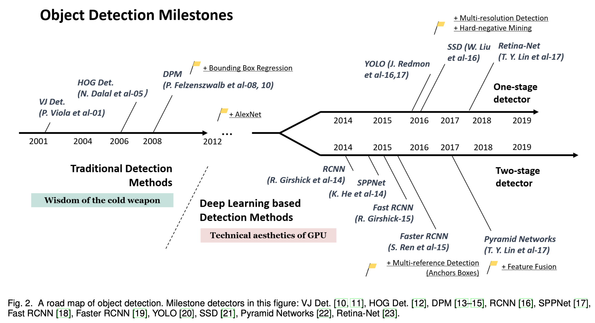
This post follows that path and records the key contributions of each algorithm along the course of development.
Traditional Detection Methods
In the earlier stage of development, the algorithms in this field were mainly traditional algorithms, that is, you had to design the relevant features yourself for machine learning.
Viola-Jones Detectors
In 2001, P. Viola and M. Jones published a classic object detection algorithm (the Viola-Jones Detector). This algorithm uses Haar-like features as input for detection on top of Adaboost, and also uses a sliding window to determine whether some region contains an object. The introduction of the sliding window adds a huge computational burden, so the authors adopted several methods to speed up the algorithm:
- Integral image: Haar features consider adjacent rectangular regions at a specific position, adding up the pixels of each rectangular region and then subtracting them (example). To compute Haar-like features, all pixels in the rectangular region need to be summed, and the rectangular regions that an image can form vary in size; if every rectangular region required traversing all its pixels and then summing, that would be very slow. The integral image means that for any point in the image, the integral image value at that point equals the sum of all pixels to the upper left of that point, with the formula:
The integral image has the following relation:
$$ I(x,y) = f(x,y)+I(x,y-1)+I(x-1,y)-I(x-1,y-1) $$Here $I$ denotes the integral image and $f$ denotes the original image. With the integral image, the sum of pixels of any rectangular region in the image can be computed:
$$ S_{abcd} = I(d)-I(b)-I(c)+I(a) $$- Feature selection: the number of Haar features extracted from an image is fairly large; the authors assume that only a small subset of these features is useful and use Adaboost for feature selection, reducing the computational burden by reducing the number of features.
- Detection cascades: to further reduce the computation, the authors do not use a traditional Adaboost classifier but cascade multiple small Adaboosts, and once some level of the cascade detects that a region is not an object, the detection of that region stops immediately.
HOG Detectors
In 2005, N. Dalal and B. Triggs proposed the HOG (Histogram of Oriented Gradients) feature extraction algorithm, which forms features by computing and collecting histograms of gradient orientations over local regions of the image. This is done because the appearance and shape of local objects in an image can be well described by the distribution of gradient or edge direction densities. Specifically, the grayscale image is divided into blocks, the gradient or edge orientation histograms of the pixels in each block are computed, and finally these histograms are combined to form the features.

The figure above shows the concrete steps a typical HOG detector performs. Gamma correction is used here to adjust the contrast of the image, reduce the influence of local shadows and illumination changes, and also suppress noise interference. Because of local illumination changes and changes in foreground-background contrast, the range of gradient magnitudes varies enormously. This requires normalizing the gradient magnitudes, and normalization can further compress the effects of illumination, shadows and edges. The authors perform the normalization by combining the features of several cells.
Deformable Part-based Model (DPM)
In 2008, P. Felzenszwalb proposed the Deformable Part Model, a component-based detection algorithm that is an extension of the HOG detector. A typical DPM model consists of a root filter and several part filters, where the root filter covers the whole object and the part filters are high-resolution templates covering parts of the object. For an object, the model formally defines it as a tuple: $(F_0,P_0,P_1,...,P_n,b)$, where $F_0$ is the root filter, $P_i$ is the model of the $i$-th part, and b represents the bias value. Each part model is represented by a triple $(F_I, v_i, d_i)$: $F_i$ is the model of the $i$-th part, $v_i$ is a two-dimensional vector specifying the anchor position of the $i$-th filter (the undeformed standard position) relative to the root coordinates, and $d_i$ is a four-dimensional vector specifying the parameters of a quadratic function that represents the deformation cost of each possible position of the part relative to the anchor position.
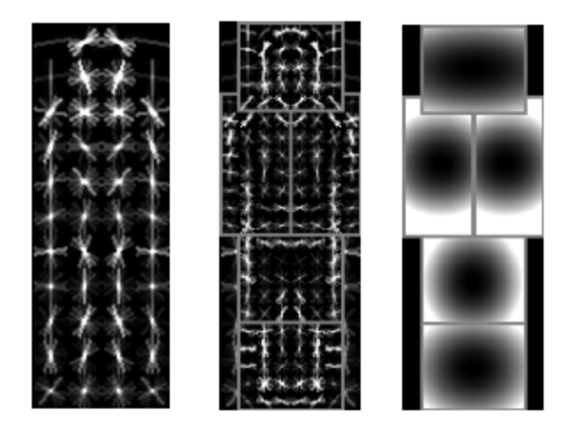
The figure above visualizes the root model, the part models and the part deformation costs. Taking a pedestrian as an example here, the left image is the root model, which roughly represents an upright pedestrian; the middle images are the part models, each of which is the part inside the rectangular box at twice the resolution of the root model, which gives better results; the right images are the deformation costs of the part models, where brighter regions indicate larger deformation cost, and the deformation cost at the standard position of the part model is 0. To reduce the complexity of the model, both the root model and the part models are axially symmetric.
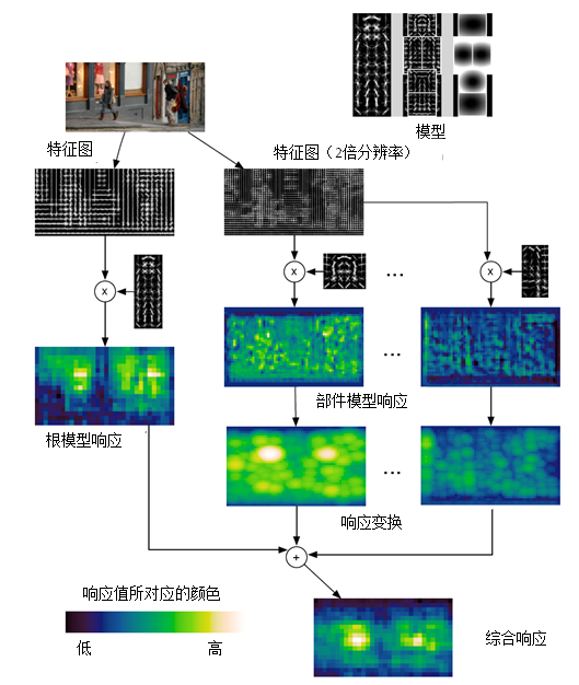
DPM uses the traditional sliding window detection approach, searching at various scales by building an image pyramid. The figure below shows the pedestrian detection process at a certain scale, that is, the matching process of the pedestrian model. The response score of a certain position with the root or part model is the inner product of that model with the features in the sub-window region anchored at that position (that is, with the top-left corner coordinates). The model can also be regarded as a filter operator, and the response score is how similar the features are to the model being matched — the more similar, the higher the score. The left side shows the detection process of the root model; in the filtered image, brighter regions represent higher response scores. The right side shows the detection process of each part model. First the feature image is matched with the model to obtain the filtered image. Then response transformation is performed. The response transformation takes the anchor position as the reference position, combines the degree to which the part model matches the features and the deformation cost of the part model relative to the standard position, and obtains the optimal part model position and response score.
Deep Learning Detection Methods
Since the AlexNet neural network achieved SOTA on Imagenet in 2012, neural networks began to receive attention. Here I introduce several key algorithms.
RCNN
In 2014, R. Girshick et al. published RCNN, the first to introduce neural network models into the object detection field. RCNN obtains a large number of candidate boxes from the original image through selective search, extracts image features for each candidate box using a convolutional neural network, then applies a linear SVM classifier to those image features, and finally obtains the class and position/size of the objects in the image.
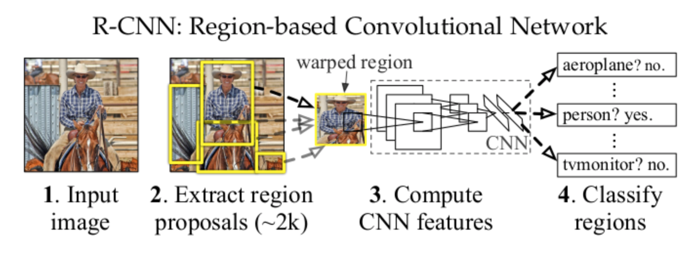
Overall the model can be divided into three parts:
- Generating class-independent candidate regions
- A convolutional network used to extract a fixed-length feature vector from each candidate region
- A set of linear SVM classifiers
SPPNet
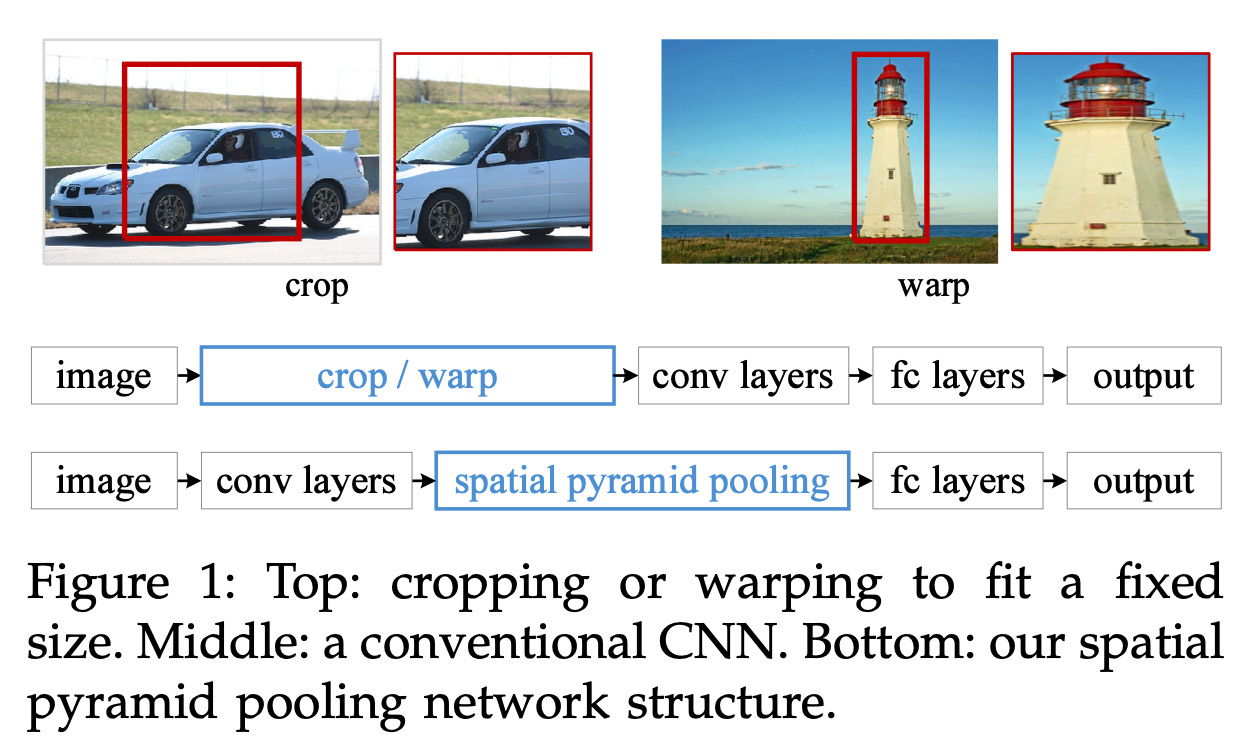
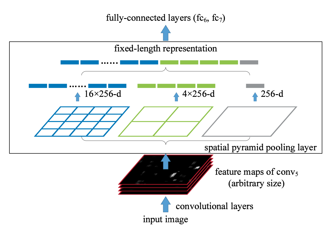
RCNN needs to resize each candidate region to a fixed size and then extract convolutional features for each region. These two steps bring some performance bottlenecks. To solve these bottlenecks, K. He et al. proposed the SPPNet model in 2014. The authors add a pooling layer before the last fully connected layer of the feature extraction network to produce a fixed output for arbitrary input, thereby solving the problem in RCNN that candidate region inputs must be of fixed size. The model also borrows the idea of the spatial pyramid, that is, dividing an image into blocks of different scales, extracting features for each block and finally concatenating them.
The figure below shows the difference between SPPNet and RCNN when handling input images of different sizes. RCNN obtains images of a fixed size by cropping or resizing and then feeds them into the convolutional neural network for computation. SPPNet, by contrast, first extracts features through a convolutional network and then obtains a fixed-size feature vector through a pooling layer as the input of the fully connected layers. The most important point is that features only need to be extracted once per image.
The main purpose of the spatial pyramid pooling layer is to produce a fixed-size output for input of any size. The idea is to first divide a feature map of any size into 16, 4 and 1 blocks, then perform max pooling on each block, and concatenate the pooled features to obtain an output of fixed dimension, satisfying the needs of the fully connected layers.
Fast RCNN
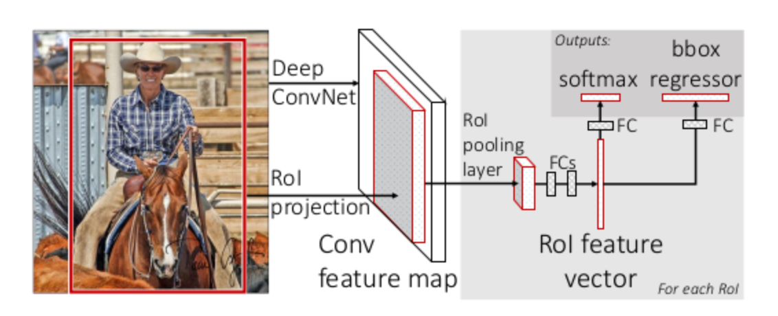
Like RCNN, SPPNet also needs to train a CNN to extract features and then train SVMs to classify those features. This requires huge storage space, and training the parts separately is also complicated. In 2015 R. Girshick introduced the Fast RCNN model, which unifies the detector and the box regressor within one framework for unified training. It takes the whole image and a set of candidate boxes as input; the model first extracts features from the whole image with a set of convolution layers and max pooling layers, then, on the extracted feature map, uses RoI pooling to extract a fixed-length feature vector for each candidate box, and then feeds it into fully connected layers that finally split into two branches for object recognition and bounding box regression. Although Fast RCNN is a big improvement over RCNN and SPPNet, the model still uses selective search to generate candidate boxes, which is the main speed bottleneck of the model.
Faster RCNN
RCNN, SPPNet and Fast RCNN all use selective search to obtain object candidate boxes, and this operation slows down the whole model. In 2015 S. Ren et al. proposed Faster RCNN, the first end-to-end deep learning object detection model running at close to real time. Its main contribution is the RPN layer. The RPN layer can generate candidate regions quickly, and it also introduces anchor boxes to select candidate regions. The rough structure is as follows, where the red box denotes the RPN layer (figure taken from the internet)
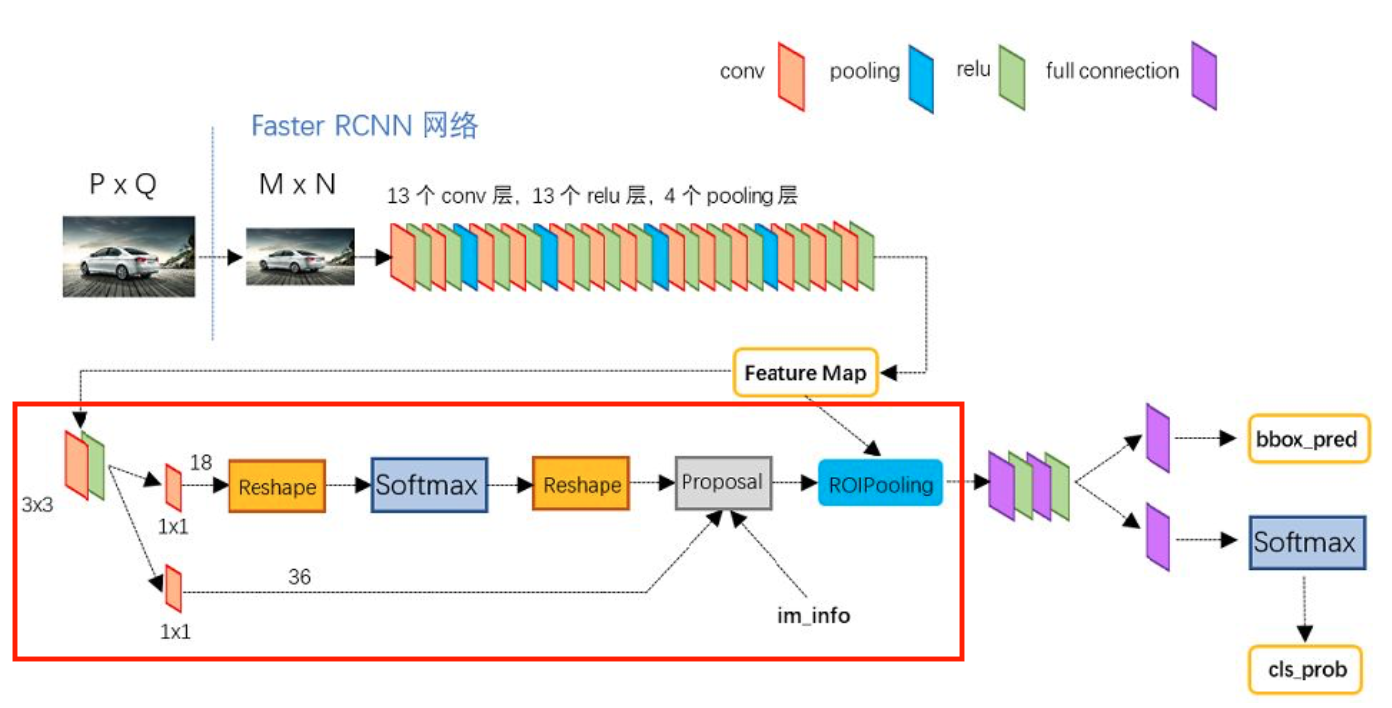
Faster RCNN abandons the traditional approach of generating candidate boxes with sliding windows and selective search and directly uses RPN to generate detection boxes. This is a huge advantage of Faster RCNN, as it can greatly speed up the generation of detection boxes; it is also from here that object detection introduced Anchors as object candidate boxes.
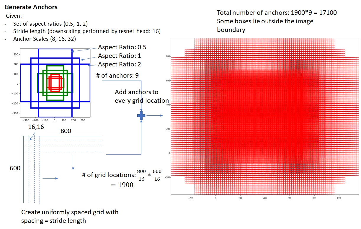
The generation of Anchors is mainly determined by two parameters: the aspect ratio and the scaling scale. For example, the figure on the right shows the nine anchor boxes Faster RCNN generates under three aspect ratios (ratios=[0.5, 1.0, 2.0]) and three scales (scales=[8, 16, 32]).
The anchor boxes are distributed over every pixel of the feature map, that is, the center of an anchor box is at the position of the feature map pixel. The resulting anchor boxes cover the whole feature map, and the anchor boxes under the same pixel have different scales, so in fact the anchor boxes introduce the multi-scale method commonly used in detection.
The rough computation is as follows:
$$ \begin{cases} w\times h = s \\ \frac{w}{h} = ratio \end{cases} \Rightarrow \begin{cases} h = \sqrt{\frac{s}{ratio}} \\ w = ratio\cdot h = \sqrt{s\cdot ratio} \end{cases} $$and further
$$ \begin{cases} h = \sqrt{\frac{s}{ratio}\cdot scale} \\ w = ratio\cdot h = \sqrt{s\cdot ratio \cdot scale} \end{cases} $$Generating anchor boxes on a feature map looks roughly like the figure below (taken from the internet):
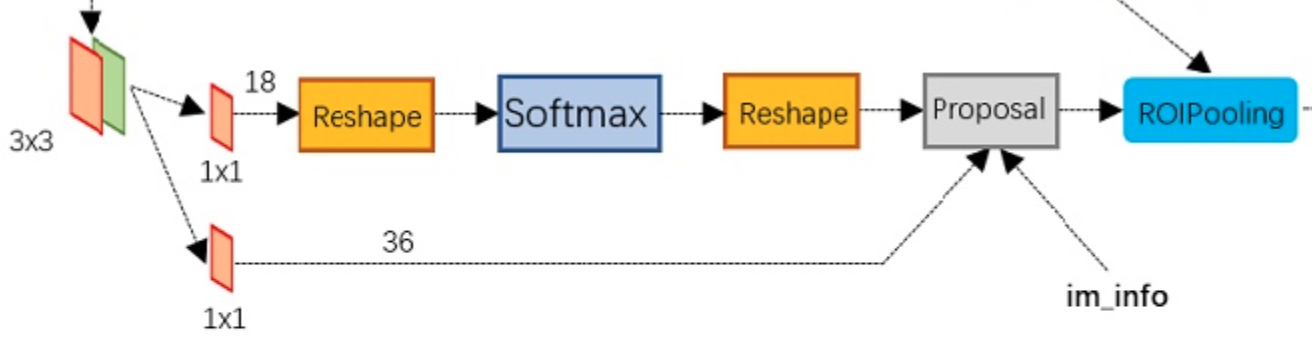
As for the RPN layer, the figure below shows the concrete structure of the RPN network. As can be seen, the RPN network is actually split into 2 lines: the upper line classifies the anchors with softmax to obtain positive and negative classes, and the lower line computes the bounding box regression offsets for the anchors to obtain accurate proposals. The final Proposal layer is responsible for combining the positive anchors and the corresponding bounding box regression offsets to obtain proposals, while removing proposals that are too small or beyond the boundary. In fact, once the whole network reaches the Proposal Layer, it has accomplished the equivalent of object localization.
Rough RPN flow:
generate anchors -> softmax classifier extracts positive anchors -> bbox reg regresses positive anchors -> Proposal Layer generates proposals
Feature Pyramid Networks (FPN)
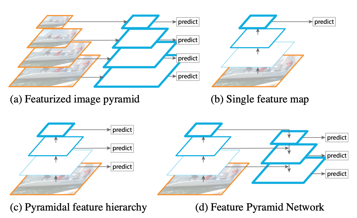
In 2017, T.-Y. Lin et al. proposed FPN on the basis of Faster RCNN. Previous neural network object detection models only extracted the features output by the topmost layer for detection, but the deeper layers of a convolutional network are good for class recognition while being bad for object localization. FPN contains a top-down network structure with lateral connections, which can be used to build high-level semantics at various scales. Basically all the various networks proposed afterwards include this structure.
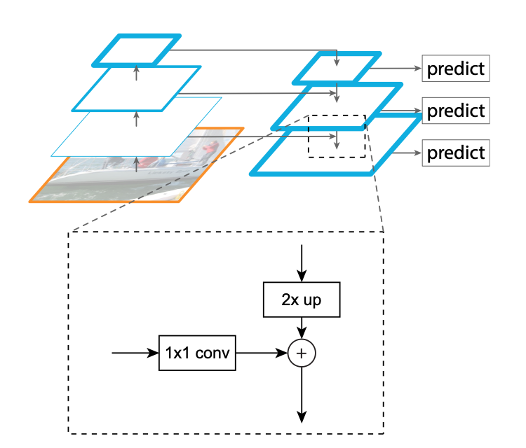
In the top-down structure of FPN, the detailed operations between network layers are as follows:
You Only Look Once (YOLO)
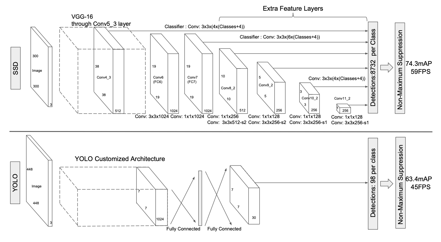
In 2015, R. Joseph proposed YOLO, the first single-stage model in the deep learning object detection field. This model divides the image into $S\times S$ grids: if the center of an object falls inside a grid cell, that grid cell is responsible for predicting the object. Each grid cell predicts $B$ bounding boxes along with the confidence of these boxes, where confidence means whether there is an object in the box and the confidence in that judgment: $Pr(Object)*IOU^{truth}_{pred}$. If there is no object in the box then $Pr(Object)$ is 0, otherwise the $IOU$ between the predicted box and the ground truth box is used as the confidence value.
The authors unify the object detection pipeline into a single neural network. This neural network uses the information of the whole image to predict the bounding boxes of objects while recognizing their classes, achieving real-time end-to-end object detection. Each bounding box predicts five variables: x, y, w, h, conf, where the first four are coordinate variables, with x and y being the center of the box and w and h denoting the width and length. Note here that the center coordinates are relative to the grid cell size while the width and height are relative to the whole image, and conf denotes the IOU between the predicted box and the positive box.
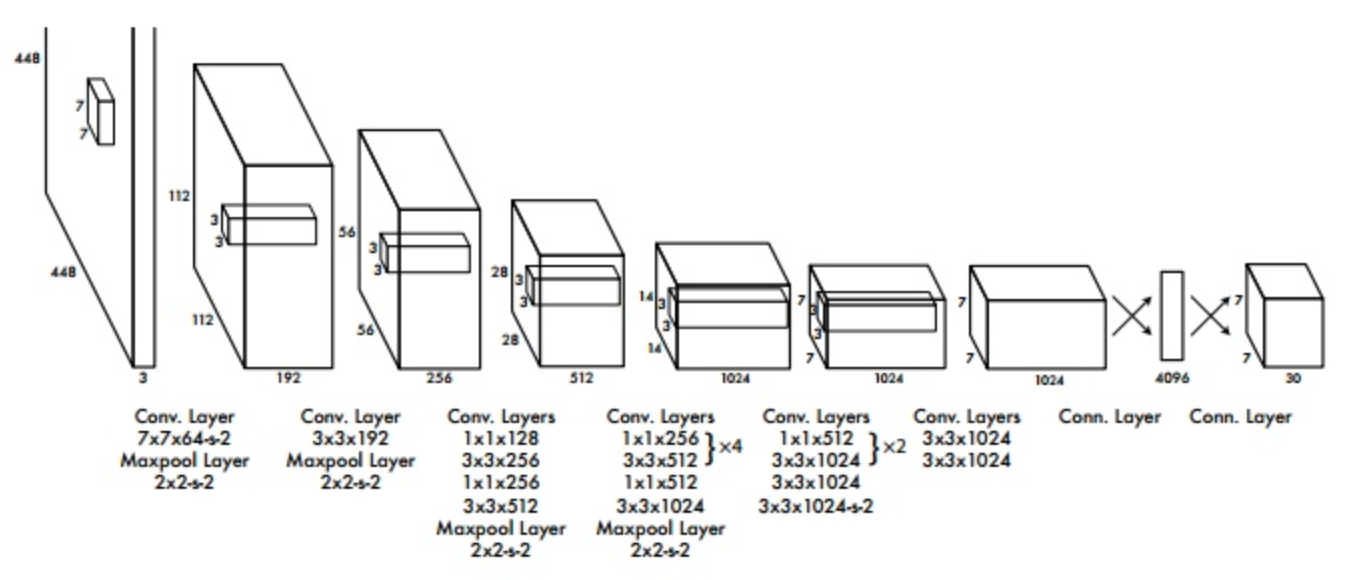
Later the authors also absorbed the characteristics of other network models and improved YOLO, releasing YOLO2 and YOLO3.
Single Shot MultiBox Detector (SSD)
Like YOLO, SSD is a single-stage detection model proposed by W. Liu et al. in 2015. The main characteristic of SSD is that it uses a multi-scale detection structure. Similar to FPN, SSD extracts feature maps from different convolution layers for detection. Since the receptive field sizes of different layers differ, this approach can take objects of different sizes into account. SSD also uses convolution layers instead of fully connected layers for the final classification and regression operations.
RetinaNet
Although single-stage models run faster than two-stage models, their accuracy is generally lower. In 2017, T.-Y. Lin et al. proposed RetinaNet. The authors believe the cause of the low accuracy of single-stage models is the extreme imbalance of positive and negative samples, and for this reason they designed the focal loss function to rebalance positive and negative samples, which is also the main contribution of RetinaNet.
The final loss function is:
$$ loss = -\alpha(1-p_t)^\gamma * log(p_t) $$where both $\alpha$ and $\gamma$ are hyperparameters. In the authors’ own experiments on their model, $\alpha=0.25$ and $\gamma=2$ worked best. This function is only used when computing the classification loss.
CornerNet
Although this last method is not in the authors’ roadmap, I personally find the anchor-free idea quite interesting, so I added it here. In single-stage object detection networks the Anchor-box approach is basically always used, but this approach requires a large number of anchors, which leads to an imbalance between positive and negative samples and reduces training efficiency; at the same time the anchor settings introduce many hyperparameters (such as number, size and aspect ratio), increasing the difficulty of network design. In 2018, Hei Law published CornerNet, which obtains the position of an object by detecting the corners of the object box, thus eliminating the need for the anchor step. The rough structure is as follows:
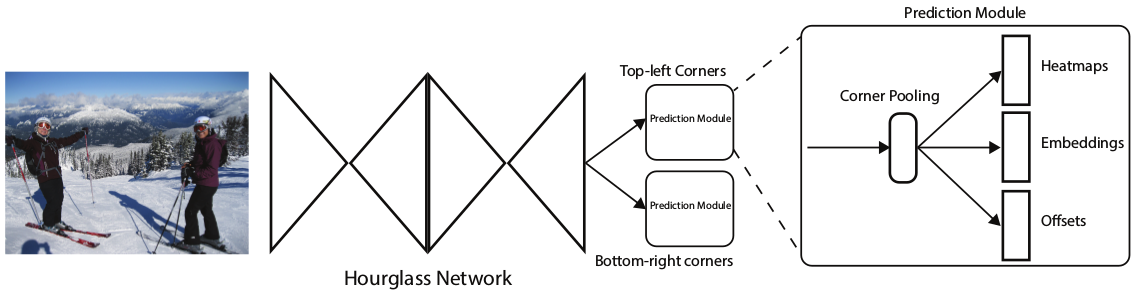
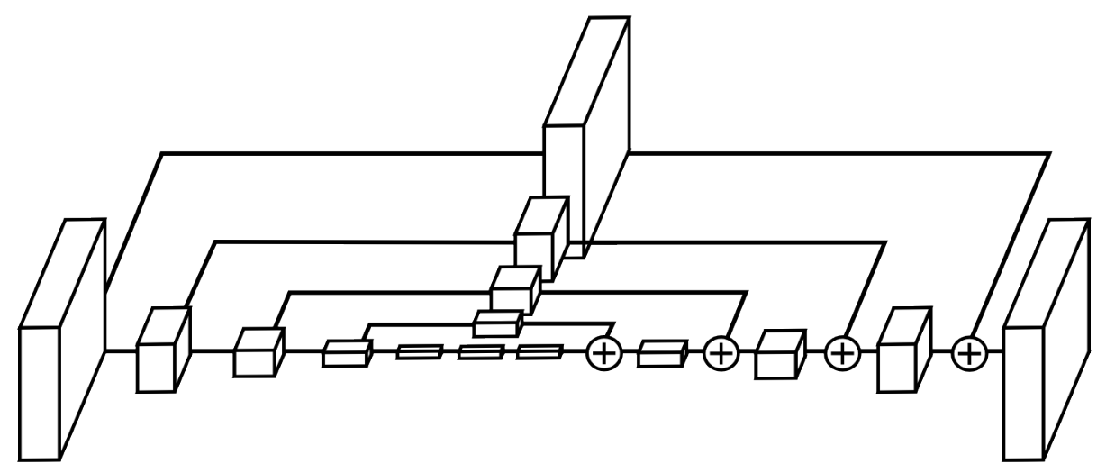
The feature extraction network here is mainly Hourglass. The Hourglass structure was proposed by Newell et al. in 2016; it mainly repeats bottom-up and top-down passes while combining the intermediate results, and in human pose estimation it can make good use of the spatial relationships of different body parts. It looks roughly like the figure below:
Corner pooling is used to localize the vertices of an object. To better suit corner detection, in object detection tasks the corners of an object often lie outside the object, so corner detection cannot rely on local features; instead, all the features along the row and the column containing that point should be scanned. The figure below takes the top-left corner as an example.
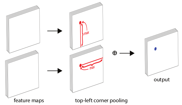
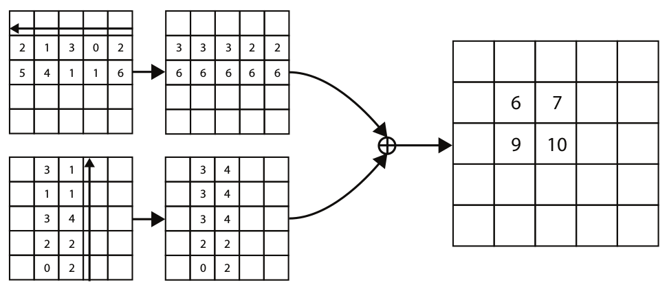
Note here that the pooling over each row and column is directional; as shown below, max pooling is performed along the row or column in the direction of the black arrow:
Datasets
Pascal VOC
In early computer vision (2005 to 2012), VOC was a very important open dataset, and the parts used most for object detection tasks are VOC07 and VOC12. VOC07 has roughly 5k training images containing 12k+ annotated objects; VOC12 has 11k training images containing 27k+ annotated objects. Both annotate the 20 classes of objects commonly seen in daily life.

ILSVRC
This dataset (2010 to 2017) contains 200 classes, and the total number of images is much larger than VOC; for example ILSVRC-14 contains 517k images and 534k annotated objects.
MS-COCO
The COCO dataset, developed from 2015 to the present, is the most challenging dataset in the current object detection field. It has fewer classes than ILSVRC but far more annotated objects than ILSVRC. The MS-COCO-17 dataset has 164k images in total, containing 897k annotated objects of 80 classes.

Open Images
The dataset released by the Open Images detection challenge, which started in 2018, is larger in scale than the COCO dataset. For the object detection task, Open Images contains 1910k images and 15440k annotated objects of 600 classes.

Metrics
Computing precision and recall:
| Actually positive | Actually negative | |
|---|---|---|
| Predicted positive | TP | FP |
| Predicted negative | FN | TN |
Precision: among the samples predicted as positive, the proportion that are truly positive.
$$ P = \frac{TP}{FP+TP} $$Recall: among the truly positive samples, the proportion that are predicted as positive.
$$ R = \frac{TP}{FN+TP} $$In the early days, the commonly used object detection evaluation metric was FPPI (false positives per image), that is, the average number of objects correctly retrieved per image:
$$ FPPI = \frac{FP}{N} $$VOC2007 introduced the AP value. The AP value is the average of the precision at different recall rates. This definition is for a single class; for multiple classes, mAP (the average of the APs of all classes) is used for evaluation.
In object detection, whether a box is correct can be determined by computing the overlap (IOU) between that box and the ground truth box and comparing it with a set overlap threshold.
$$ IOU(A,B) = \frac{A\cap B}{A\cup B} $$By setting different IOU thresholds, the strictness of the evaluation criterion can be changed. After 2014, the MS-COCO dataset’s evaluation criterion defines the AP value as the average AP over IOU thresholds from 0.5 to 0.95.
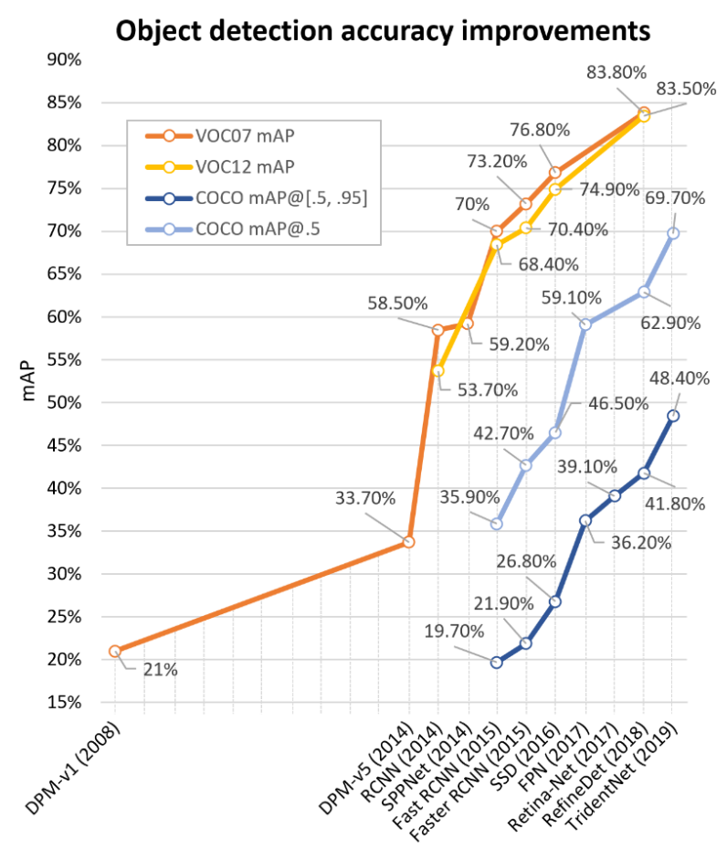
The figure below lists the accuracy of various detection algorithms:
Challenge
Lightweight object detection: the overall performance of object detection algorithms still lags somewhat behind human vision, and the gap in speed is even more obvious. So lightweight model design is an important research direction;
Detection meets AutoML: today’s detection models are increasingly complex and also depend on people’s experience. Network architecture search can greatly reduce the extent to which people are involved in model structure design; models in this direction already exist, such as Efficientdet, and it will be a development direction in the future as well;
Weakly supervised detection: from the development of datasets we can see that detection models have enormous data requirements, while annotating datasets consumes a lot of manpower and time, and annotations by different people have some bias. So how to achieve weakly supervised object detection is an important problem;
Detection in videos: how to perform object detection in videos is also an important problem in the detection field. The usual approach is to detect every frame of the video, but this ignores the correlation information between video frames. Mining the spatial and temporal correlations in videos is very important for object detection in videos
Reference
This post is mainly based on the following articles; for more detailed content see the original paper: Object Detection in 20 Years: A Survey
Rapid object detection using a boosted cascade of simple features
A discriminatively trained, multiscale, deformable part model
Rich feature hierarchies for accurate object detection and semantic segmentation
Spatial Pyramid Pooling in Deep Convolutional Networks for Visual Recognition
Faster R-CNN: Towards Real-Time Object Detection with Region Proposal Networks