Mathematics is the queen of the sciences. — Gauss
Probabilistic undirected graphical model
Before understanding the probabilistic undirected graphical model, let us look at the definition of the probabilistic graphical model (PGM): it is a probability distribution represented by a graph. Suppose there is a joint probability distribution $P(Y)$, where $Y\in \mathcal{Y}$ is a group of random variables, and the probability distribution $P(Y)$ is represented by an undirected graph $G=(V, E)$; that is, in graph $G$, a node $v\in V$ represents a random variable $Y_v$, $Y_v=(Y_v)_{v\in V}$; an edge $e\in E$ represents the probabilistic dependency between random variables.
Given a joint probability distribution $P(Y)$ and the undirected graph $G$ representing it. Three properties are explained below.
Pairwise Markov property
$$ P(Y_u,Y_v\mid Y_O) = P(Y_u\mid Y_O)P(Y_v\mid Y_O) $$where $u$ and $v$ are any two nodes in the undirected graph not connected by an edge, with corresponding random variables $Y_u$ and $Y_v$, and $O$ is all the other nodes in the undirected graph besides $u$ and $v$, with the corresponding group of random variables $Y_O$. That is, given the group of random variables $Y_O$, the random variables $Y_u$ and $Y_v$ are conditionally independent.
Local Markov property
$$ P(Y_u,Y_O\mid Y_W) = P(Y_v\mid Y_W)P(Y_O\mid Y_W) $$where $v\in V$ is any node in the undirected graph $G$ with corresponding random variable $Y_v$, $W$ are all the nodes connected to $v$ by edges with the corresponding group of random variables $Y_W$, and $O$ are all the other nodes besides $v$ and $W$, with the corresponding group of random variables $Y_O$. That is, given the group of random variables $Y_W$, the random variable $Y_v$ is independent of the group of random variables $Y_O$.
Global Markov property
$$ P(Y_A,Y_B\mid Y_C) = P(Y_A\mid Y_C)P(Y_B\mid Y_C) $$where the node sets $A$ and $B$ are any node sets in the undirected graph $G$ separated by the node set $C$, with corresponding groups of random variables $Y_A$, $Y_B$ and $Y_C$. That is, given the group of random variables $Y_C$, the groups of random variables $Y_A$ and $Y_B$ are conditionally independent.
The three definitions above are equivalent.
Combining the above, here is the definition of a probabilistic undirected graphical model. Suppose there is a joint probability distribution $P(Y)$ represented by an undirected graph $G=(V,E)$; in graph $G$, nodes represent random variables and edges represent the dependencies between random variables. If the joint probability distribution $P(Y)$ satisfies the pairwise, local or global Markov property, this joint probability distribution is called a probabilistic undirected graphical model, or a Markov random field (MRF).
Factorization
The core of a probabilistic graphical model is computing the joint probability distribution
A subset of nodes in an undirected graph $G$ in which every two nodes are connected by an edge is called a clique. If $C$ is a clique of the undirected graph $G$ and no other node of $G$ can be added to it to make it a larger clique, then this $C$ is called a maximal clique.
The operation of expressing the joint probability distribution of a probabilistic undirected graphical model as the product of functions of the random variables on its maximal cliques is called the factorization of the probabilistic undirected graphical model.
Given a probabilistic undirected graphical model, let its undirected graph be $G$, let $C$ be a maximal clique of $G$, and let $Y_c$ denote the random variable corresponding to $C$. By the Hammersley-Clifford theorem we have that, if and only if the joint probability density of the random variables is strictly positive, the probabilistic undirected graphical model is equivalent to a Gibbs random field (GRF). And the joint probability distribution $P(Y)$ of the GRF can be written as the product of functions $\Psi_C(Y_C)$ over all maximal cliques $C$ of the graph, namely:
$$ \begin{aligned} P(Y) & = \frac{1}{Z}\prod_C\Psi_C(Y_C) \\ Z & = \sum_Y\prod_C\Psi_C(Y_C) \end{aligned} $$where $Z$ is the normalization factor, used to ensure that $P(Y)$ forms a probability distribution, that is, sums to 1. The function $\Psi_C(Y_C)$ is called the potential function. Here the potential function is required to be strictly positive; for convenience it is usually defined as an exponential function:
$$ \Psi_C(Y_C) = exp\{-E(Y_C)\} $$Conditional random field
Definition: Let $X$ and $Y$ be random variables and $P(X\mid Y)$ be the conditional probability distribution of $Y$ given $X$. If the random variable $Y$ constitutes a Markov random field represented by an undirected graph $G=(V,E)$, that is,
$$ P(Y_v\mid X,Y_w,w\ne v) = P(Y_v\mid X,Y_w,w\sim v) $$holds for any node $v$, then $P(Y\mid X)$ is called a conditional random field. Here $w\sim v$ denotes all nodes $w$ in graph $G=(V,E)$ connected to node $v$ by edges, $w\ne v$ denotes all nodes other than node $v$, and $Y_v$, $Y_u$ and $Y_w$ are the random variables corresponding to nodes $v$, $u$ and $w$.
$X$ and $Y$ can have different graph structures, but in general they are assumed to have the same graph structure, which gives the linear chain conditional random field. Let $X=(X_1,X_2,\cdots,X_n)$ and $Y=(Y_1,Y_2,\cdots,Y_n)$ both be random variable sequences represented by linear chains; if, given the random variable sequence $X$, the conditional probability distribution $P(Y\mid X)$ of the random variable sequence $Y$ constitutes a conditional random field, that is, it satisfies the Markov property
$$ P(Y_i\mid X,Y_1,\cdots,Y_{i-1},Y_{i+1},\cdots,Y_n) = P(Y_i\mid X,Y_{i-1},Y_{i+1}) \\ i=1,2,\cdots,n \ (only one side is considered when i=1 and n) $$then $P(Y\mid X)$ is called a linear chain conditional random field, which is also a log linear model.
Parameterized form of the linear chain conditional random field
For the linear chain conditional random field $P(Y\mid X)$, given that the random variable $X$ takes the value $x$, the conditional probability of the random variable $Y$ taking the value $y$ has the following parameterized form:
$$ P(y\mid x) = \frac{1}{Z(x)}exp\left(\sum_{i,k}\lambda_kt_k(y_{i-1},y_i,x,i)+\sum_{i,l}\mu_ls_l(y_i,x,i)\right) $$where
$$ Z(x) = \sum_yexp\left(\sum_{i,k}\lambda_kt_k(y_{i-1},y_i,x,i)+\sum_{i,l}\mu_ls_l(y_i,x,i)\right) $$In the formulas, $t_k$ and $s_l$ are feature functions, $\lambda_k$ and $\mu_l$ are the corresponding weights, and $Z(x)$ is the normalization factor; the summation runs over all possible output sequences. $t_k$ is a feature function defined on edges, called a transition feature, which depends on the current and the previous position; $s_l$ is a feature function defined on node $l$, called a state feature, which depends on the current position. Both feature functions depend on the position and are local feature functions, and they generally take the value 1 or 0, being 1 when the condition is met and 0 otherwise.
Simplified form of the linear chain conditional random field
Suppose there are $K_1$ transition features and $K_2$ state features, with $K=K_1+K_2$; then
$$ \begin{aligned} & f_k(y_{i-1},y_i,x,i) = \begin{cases} t_k(y_{i-1},y_i,x,i), &\ k=1,2,\cdots, K_1 \\ s_l(y_i,x,i), &\ k=K_1+l;\ l=1,2,\cdots, K_2 \end{cases} \\ & \Rightarrow f_k(y,x) = \sum_{i=1}^nf_k(y_{i-1},y_i,x,i), \qquad k=1,2,\cdots,K \end{aligned} $$Likewise, $w_k$ is used to express the weights uniformly:
$$ w_k = \begin{cases} \lambda_k, &\ k=1,2,\cdots,K_1 \\ \mu_l, &\ k=K_1+l;\ l=1,2,\cdots,K \end{cases} $$In summary we obtain:
$$ P(y\mid x) = \frac{1}{Z(x)}exp\sum_{k=1}^{K}w_kf_k(y,x) \\ Z(x) = \sum_yexp\sum_{k=1}^Kw_kf_k(y,x) $$If $w=(w_1,w_2,\cdots,w_K)^T$ denotes the weight vector and $F(y,x)=(f_1(y,x),f_2(y,x),\cdots,f_K(y,x))^T$ denotes the global feature vector, then the formula above can be expressed further as follows:
$$ P_w(y\mid x) = \frac{exp(w\cdot F(y,x))}{Z_w(x)} \\ Z_w(x) = \sum_yexp(w\cdot F(y,x)) $$Matrix form of the linear chain conditional random field
For each position $i=1,2,\cdots,n+1$ of the input sequence $x$, define an $m$-order matrix ($m$ being the number of values $y_i$ can take):
$$ M_i(x) = [M_i(y_{i-1},y_i\mid x)] \\ M_i(y_{i-1},y_i\mid x) = exp(W_i(y_{i-1},y_i\mid x)) \\ W_i(y_{i-1},y_i\mid x) = \sum_{k=1}^Kw_kf_k(y_{i-1},y_i,x,i) $$Combining the simplified form above with the $m$-order matrix here gives
$$ \begin{aligned} & exp\sum_{k=1}^Kw_k\sum_{i=1}^nf_k(y_{i-1},y_i,x,i) \\ = & exp\sum_{k=1}^K\sum_{i=1}^nw_kf_k(y_{i-1},y_i,x,i) \\ = & exp\sum_{i=1}^n\sum_{k=1}^Kw_kf_k(y_{i-1},y_i,x,i) \\ = & exp\sum_{i=1}^nW_i(y_{i-1},y_i\mid x) \\ = & \prod_{i=1}^nexp(W_i(y_{i-1},y_i\mid x)) \\ = & \prod_{i=1}^nM_i(y_{i-1},y_i\mid x) \\ = & \prod_{i=1}^{n+1}M_i(y_{i-1},y_i\mid x) \qquad (adding the start state and the stop state) \end{aligned} $$In the last step of the derivation above, $y_0=start$ and $y_{n+1}=stop$ denote the start state and the stop state respectively. This gives:
$$ P_w(y\mid x) = \frac{1}{Z(x)}\prod_{i=1}^{n+1}M_i(y_{i-1},y_i\mid x) \\ Z_w(x) = (M_1(x)M_2(x)\cdots M_{n+1}(x))_{start,stop} $$The normalization factor $Z_w(x)$ is the sum of the unnormalized probabilities $\prod_{i=1}^{n+1}M_i(y_{i-1},y_i\mid x)$ of all paths $y_1y_2\cdots y_n$ through the states from start to stop.
Some applications
CRF is suited to situations where there are dependencies between contextually related samples. It has a great many applications in the NLP field; for the CV field, limited as my knowledge is, the applications I have seen so far are all in the image segmentation field. Segmentation is pixel-level, so every pixel in the image is a node $x$ and the corresponding label is $y$; the relationships between pixels can be represented as edges. Since the surrounding pixels have a much greater influence on the label than other pixels, we can infer the label of the target pixel from the labels of the surrounding pixels, and this whole setup forms a conditional random field.
DenseCRF
DenseCRF is a fully connected conditional random field; what differs from an ordinary conditional random field is that the pairwise potential function describes the relationship between every pixel and all other pixels.
From the earlier definition we know that the potential function of a CRF is $\Phi_c(X_c)=e^{-E(X_c)}$ (other functions can be chosen, but $\Phi_c(X_c) > 0$ must always hold), where $E(X_c)$ is the energy function; for the segmentation field the energy function is generally expressed as follows:
$$ E(X) = \sum_i\phi_u(x_i)+\sum_{iwhere $\mu(x_i,x_j$ is the label compatibility, which constrains the propagation between pixels: energy can only propagate when the labels are the same. $w^{(m)}$ is a weight parameter and $k^{(m)}(f_i,f_j)$ is the Gaussian kernel feature function:
$$ k^{(m)}(f_i,f_j) = w^{(1)}exp\left(-\frac{\vert p_i-p_j\vert^2}{\theta_{\alpha}^2}-\frac{\vert I_i-I_j\vert^2}{2\theta_{\beta}^2}\right) + w^{(2)}exp\left(-\frac{\vert p_i-p_j\vert^2}{2\theta_{\gamma}^2} \right) $$The formula expresses the similarity between different pixels as features, where the first term is the appearance kernel, mainly taking into account the fact that nearby pixels with similar colors very likely belong to the same class, and the second term is the smoothness kernel, mainly used to eliminate some small isolated pixel regions (that is, noise).
The input of the unary potential function is the probability distribution map, that is, the result obtained by applying softmax to the feature map output by the model; the position information and color information in the pairwise potential function are provided by the original image.
CRF is usually placed after a convolutional neural network to smooth the output of the network. Generally speaking, the greater the energy the lower the probability that the substance exists, and the smaller the energy the higher the probability that it exists. So we need to minimize this energy function $E(X)$ to obtain the most likely segmentation result for the current image. To save computation, this minimization is generally done through the mean field approximation, that is, minimizing the KL divergence between the approximate distribution and the target distribution. As the formulas are numerous, they are not derived here; see the supplementary material of the DenseCRF paper for details.
CRFasRNN
The DenseCRF above is added after the convolutional model as a post-processing step, whereas CRFasRNN integrates the CRF iterative process into the convolutional network to form an end-to-end model.
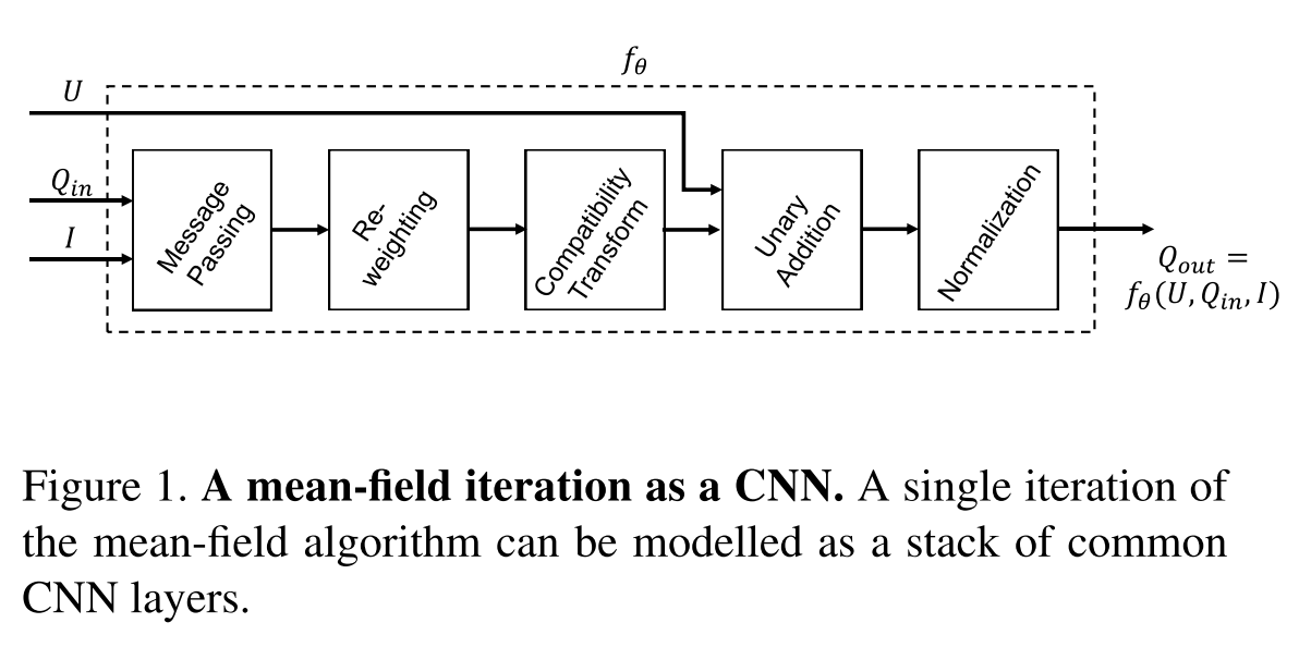
Similar to DenseCRF, the paper also uses the mean field approximation to minimize the energy function. Since the computation involves only addition and multiplication, the computation can be expressed with a convolution-like structure and thus merged into the convolutional network. To obtain more accurate results, the authors also incorporate the iterative process, that is, the iterative computation is performed inside this “convolution layer”, similar to the operation of an RNN.
The figure below shows the iterative algorithm of the mean field approximation
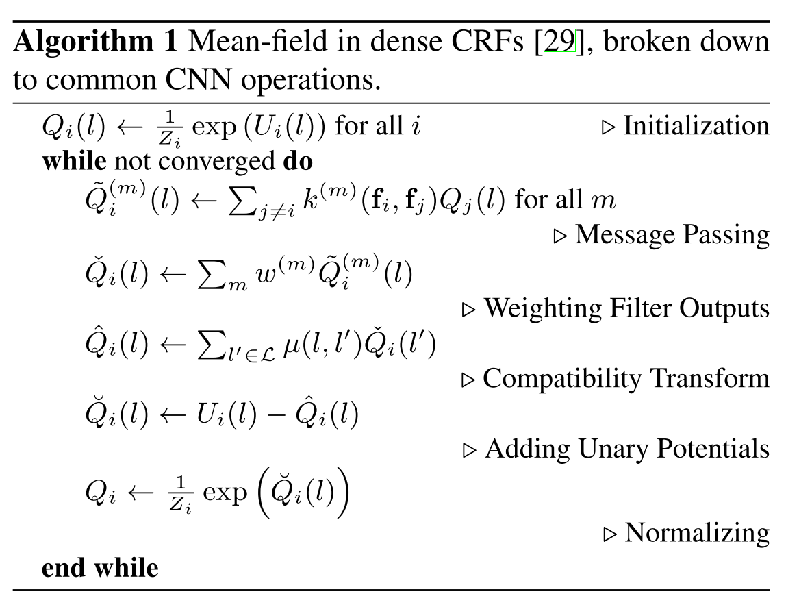
The steps in the mean field approximation computation are converted as follows:
The rough final structure of CRFasRNN:
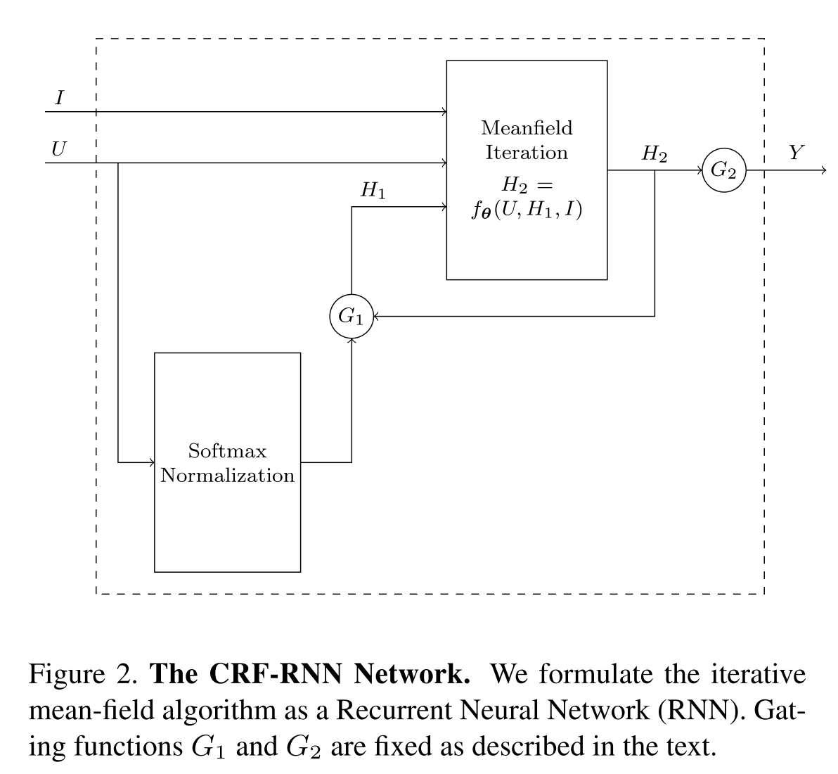
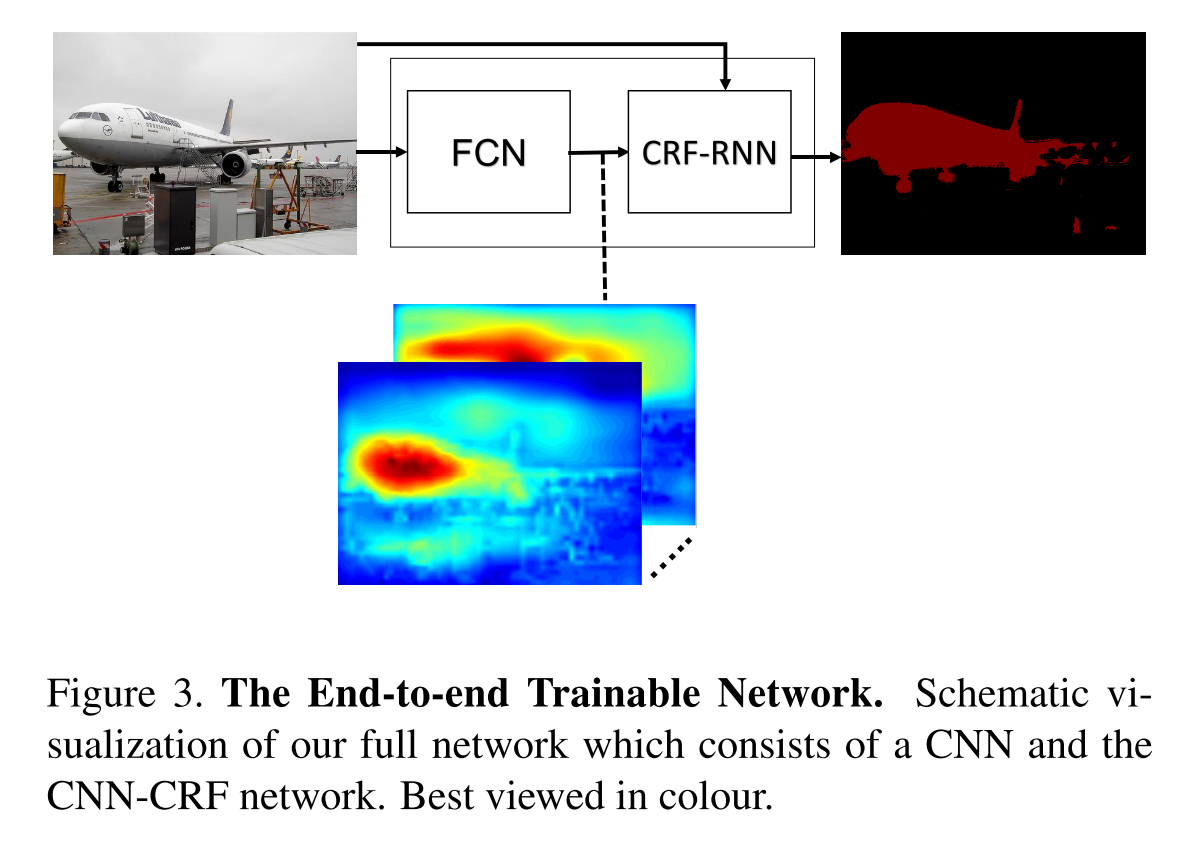
where
$$ \begin{aligned} H_1(t) & = \begin{cases} softmax(U), &\ t=0 \\ H_2(t-1), &\ 0That is the conditional random field and some of its applications that I have been studying lately. The application of probabilistic graphical models in image segmentation does not stop here — there are several more that I will update later as the situation allows. :>
Reference
Statistical Learning Methods, Li Hang
Efficient Inference in Fully Connected CRFs with Gaussian Edge Potentials
Efficient Inference in Fully Connected CRFs with Gaussian Edge Potentials Supplementary Material