Make it dynamic.
Dynamic Convolution
Ordinary static convolution applies the same kernel to all input images, whereas dynamic convolution adapts to different images and processes them with more suitable convolution parameters, which increases the expressive power of the model without increasing network depth or width.
Dynamic convolution dynamically aggregates multiple parallel convolution kernels according to attention. The attention dynamically adjusts the weight of each kernel according to the input, thereby producing an adaptive dynamic convolution. Because the attention is a function of the input, dynamic convolution is no longer a linear function. Superimposing kernels in a nonlinear way through attention gives stronger representational power. The rough structure is as follows:
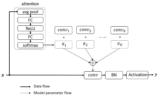
As shown above, compared with ordinary static convolution, dynamic convolution introduces two extra computations: the attention module and the superposition of the kernels. But the computation of these two parts is very small, and superposing multiple kernels is also very efficient computationally. The small extra computation together with the significant gain in expressive power makes dynamic convolution very suitable for lightweight neural networks.
Restricting the attention values simplifies the learning of the attention model and also narrows the value space of the superposed kernel. The paper restricts the attention values to between 0 and 1 with all attentions summing to 1. As shown below, if 3 kernels are used, restricting the attention to between 0 and 1 confines the superposed kernel to the two triangular pyramids, and having the attentions sum to 1 further confines the superposed kernel to the triangle with these three kernels as vertices. For these two constraints the paper uses softmax.
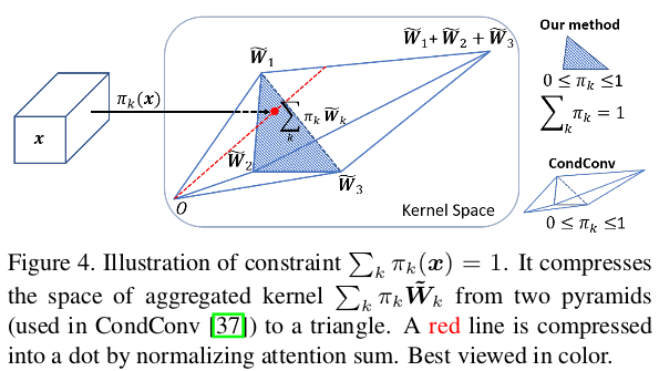
In addition, keeping the attention values close to a uniform distribution helps multiple kernels learn simultaneously in the early stage of training. Because softmax outputs sparser attention, the paper uses temperature annealing to improve model accuracy (attention close to a uniform distribution can be achieved by using a larger temperature).
Dynamic ReLU
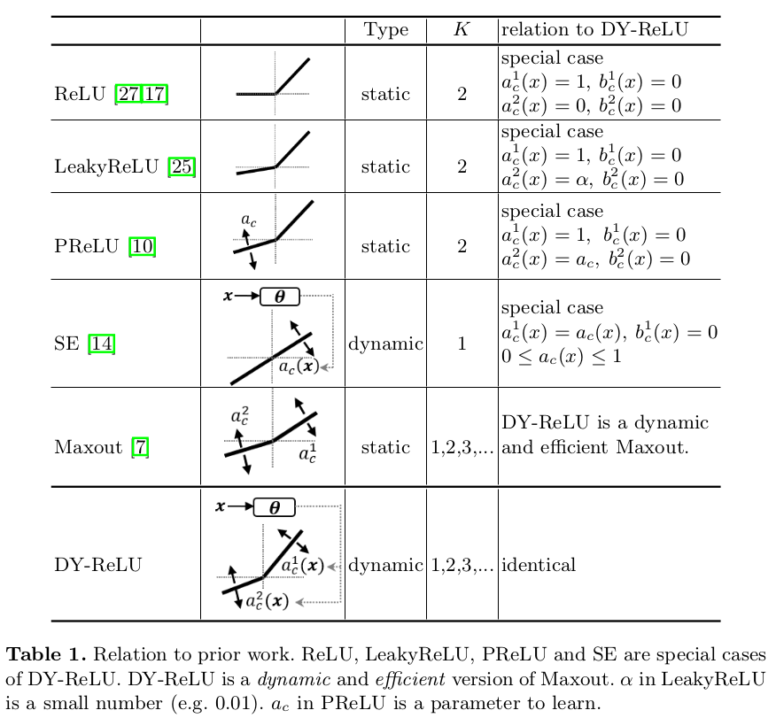
Usually the parameters of ReLU and of some of its improved versions (Leaky ReLU, PReLU) are fixed, so the paper proposes dynamic ReLU. It can adjust the parameters of ReLU according to the input features.
The original ReLU is $y = \max \lbrace x,0\rbrace$; for the $c$-th feature of the input vector $x$, the activation value is computed as $y_c = \max \lbrace x_c, 0\rbrace$. ReLU can be written uniformly as the piecewise linear function $y_c = \max\limits_k \lbrace a^k_cx_c+b^k_c\rbrace$. Based on the formula above, DY-ReLU can be defined as the maximum of several ($K$) linear functions. That is, for all inputs $x=\lbrace x_c\rbrace$ the adaptive $a^k_c$, $b^k_c$ satisfy:
$$ \begin{aligned} y_c &= f_{\theta(x)}(x_c) \\ &= \max\limits_{1\le k\le K}\{a^k_c(x)x_c+b^k_c(x)\} \end{aligned} $$The parameters $(a^k_c,b^k_c)$ are the output of the hyper function $\theta(x)$:
$$ \theta(x) = [a^1_1,\dots,a^1_C,\dots,a^K_1,\dots,a^K_C,b^1_1,\dots,b^1_C,\dots,b^K_1\dots,b^K_C]^T $$where $C$ is the number of channels, and the activation parameters $(a^k_c, b^k_c)$ are not only related to $x_c$ but also to $x_{j\ne c}$, that is, they are also related to the inputs of other channels.
The paper implements the hyper function with a lightweight network similar to the SE module. For an input $x$ of size $C\times H\times W$, global average pooling is first used to compress the spatial information, then two fully connected layers are applied (with ReLU in between), and finally a normalization layer is applied, which uses $2\sigma(x)-1$ to constrain the result between -1 and 1 ($\sigma$ is the Sigmoid function). The final output consists of $2KC$ elements, corresponding to the residuals of $a_{1:C}^{1:K}$ and $b_{1:C}^{1:K}$, that is, $\Delta a_{1:C}^{1:K}$ and $\Delta b_{1:C}^{1:K}$. The final output is the sum of the initial values and the residuals:
$$ \begin{aligned} a^k_c(x) &= \alpha^k+\lambda_a\Delta a^k_c(x) \\ b^k_c(x) &= \beta^k+\lambda_b\Delta b^k_c(x) \end{aligned} $$where $\alpha^k$ and $\beta^k$ are the initial values of $a^k_c$ and $b^k_c$. $\lambda_a$ and $\lambda_b$ are scalars used to control the magnitude of the residuals. $\alpha^k$, $\beta^k$, $\lambda_a$ and $\lambda_b$ are hyperparameters independent of the channel; by default $\lambda_a=1.0$ and $\lambda_b=0.5$, so the default hyperparameters are $\alpha^{1:K}$ and $\beta^{1:K}$.
The paper also gives three implementations of DY-ReLU, roughly as follows:

DY-ReLU-A
Spatial and channel-shared. The final output size is $2K$; the computation is relatively simple and the expressive power is also weaker.
DY-ReLU-B
Spatial-shared and channel-wise. The final output size is $2KC$, that is, $2K$ per channel.
DY-ReLU-C
Spatial and channel-wise. Every element of every channel has an independent activation function, so the final output has $2KHWC$ parameters, and using a fully connected layer directly would bring a lot of extra computation. The paper improves on this as shown in the figure above: the spatial position is decoupled into another attention branch, and finally the channel parameters $a_{1:C}^{1:K}$ and $b_{1:C}^{1:K}$ are multiplied by the spatial position attention $\pi_{1:HW}$. The spatial position attention is computed simply with $1\times 1$ convolution and a normalization method, using a constrained softmax function:
$$ \pi_{h,w} = \min \{\frac{\gamma\exp (z_{h,w}/\tau)}{\sum_{h,w}\exp (z_{h,w}/\tau)}, 1\} $$where $\gamma$ is a scalar used to amplify the softmax values and prevent vanishing gradients; the paper sets it to $\frac{HW}{3}$. $z_{h,w}$ is the output of the $1\times 1$ convolution. $\tau$ is the temperature, and a large temperature (such as $\tau$ = 10) can be used to prevent the spatial position attention from being too sparse in the early stage of training.