The multi-object tracking frameworks commonly used in industry at present.
SORT
This algorithm is based on an object detection network (Faster Rcnn) and makes use of the Kalman filter and the Hungarian algorithm (or the KM algorithm), greatly improving the speed of multi-object tracking. The rough pipeline is as follows:
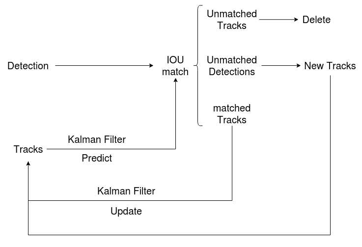
The object detection algorithm obtains the object boxes Detections of the current frame, the Kalman filter obtains the Tracks of the current frame, and IOU matching is performed between the Detections and the Tracks. The final results fall into three categories:
- Unmatched Tracks: that is, Tracks that are partly unmatched. If the mismatch persists for $T_{lost}$ times, the object is deleted.
- Unmatched Detections: that is, Detections that are partly unmatched. A new Track needs to be assigned to such a Detection.
- matched Tracks: this part means a match has been found, and is used to update the Kalman filter.
The Kalman filter can predict the state of the object boxes of the next frame from the state of the Tracks, and the update uses the observations (the matched Tracks) and the estimates to update the states of all Tracks.
DeepSORT
Compared with SORT, DeepSORT improves the performance of SORT by integrating appearance information and using cascaded matching. This allows the model to better handle objects that are occluded for a long time, greatly reducing the measured ID switch metric. Appearance information refers to the features corresponding to an object; in the paper, a deep association metric trained on a large person re-identification dataset is used to extract appearance features (borrowing models from the ReID field). The overall pipeline is roughly as follows:
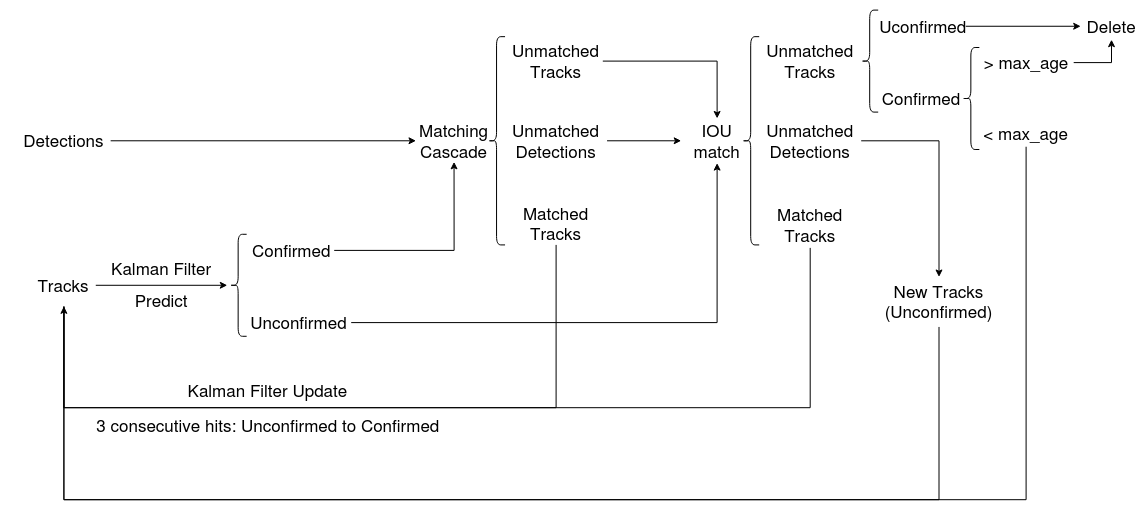
Each track maintains a variable $h$ recording the difference between the current frame and the frame of the last successful match; when a track matches a detection, $h$ is set to 0. When $h$ exceeds a preset threshold $A_{max}$, the track is considered terminated (that is, a track that has not been matched for a long time is considered finished). For detections that were not matched successfully, they may be new tracks or false detections. The paper sets an Unconfirmed state to distinguish them: when the track is matched successfully for $n\_init$ consecutive frames (set to 3 in the paper), its state is changed to Confirmed; otherwise the track is deleted. The transitions between states are as follows:

For matching, the algorithm uses both the appearance model and the motion model to compute the similarity and obtain the cost matrix, and uses a gating matrix to limit overly large values in the cost matrix.
The motion model uses the squared Mahalanobis distance between the detection and the track to characterize the degree of motion matching:
$$ \begin{aligned} d^{(1)}(i,j) &= (d_j-y_i)^TS_i^{-1}(d_j-y_i) \\ b^{(1)}_{i,j} &= I[d^{(1)}(i,j) \le t^{(1)}] \end{aligned} $$where $d_j$ denotes the $j$th detection, $y_i$ denotes the $i$th track, and $S_i^{-1}$ represents the covariance of $d$ and $y$. $b_{i,j}^{(1)}$ is an indicator that uses the 0.95 quantile of the chi-square distribution ($t^{(1)}=9.4877$) as the threshold; below the threshold the match is considered successful.
Mahalanobis distance:
The Mahalanobis distance represents the covariance distance of data, and is an effective way to compute the similarity between two unknown sample sets. Unlike the Euclidean distance, it takes into account the correlations between the various characteristics of the data.
For a multivariate vector $x=(x_1,x_2,\dots,x_p)^T$ with mean $\mu=(\mu_1,\mu_2,\dots,\mu_p)^T$ and covariance matrix $\Sigma$, its Mahalanobis distance is:
$$ D_M(x) = \sqrt{(x-\mu)^T\Sigma^{-1}(x-\mu)} $$The covariance matrix is square, with a dimension matching that of the samples.
The appearance model uses cosine distance to measure the distance between appearance features (a feature vector is extracted by the model, and cosine distance is used for comparison):
$$ \begin{aligned} d^{(2)}(i,j) &= min\{1-r_j^Tr_k^{(i)}\vert r_k^{(i)}\in R_i\} \\ b^{(2)}_{i,j} &= I[d^{(2)}(i,j) \le t^{(2)}] \end{aligned} $$where $r_j^Tr_k^{(i)}$ computes the cosine similarity (cosine distance = 1 - cosine similarity). Matching with motion information alone in SORT leads to fairly serious ID switching; introducing the appearance model and cascaded matching can alleviate this problem. $b_{i,j}^{(2)}$ is an indicator: if the cosine distance is below the threshold the match is considered successful, and this threshold is a hyperparameter (set to 0.2 in the paper). Since a track that is too long causes the appearance to change, continuing to use this minimum cosine distance as a metric carries risk, so the paper only computes the minimum cosine distance over the most recent $L_k=100$ detections of a track.
The overall matching cost is obtained by weighting the motion model and the appearance model:
$$ c_{i,j} = \lambda d^{(1)}(i,j)+(1-\lambda)d^{(2)}(i,j) \tag{5} $$$\lambda$ is a hyperparameter; considering that the camera may move, the authors set it to 0.
The gating matrix is computed as follows:
$$ b_{i,j} = \prod_{m=1}^2b^{(m)}_{i,j} \tag{6} $$$b_{i,j}$ is also an indicator; only when $b_{i,j}=1$ can a preliminary match be made.
Another method proposed by DeepSORT to deal with objects occluded for a long time is cascaded matching. When a track has been occluded for a long time, the Kalman filter keeps predicting without being able to update. In this situation, when two tracks compete for the same detection, the track that has been occluded longer often yields a smaller Mahalanobis distance and thus is more likely to match the detection, which interferes with the continuity of tracks. So cascaded matching is used to ensure that each matching round considers tracks with the same occlusion time, and tracks with less occlusion time are considered first. The algorithm is roughly as follows:
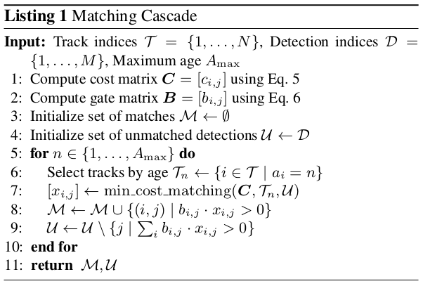
In the final stage of matching, an IOU-based matching is also performed on the Unconfirmed and unmatched tracks with age=1. This can alleviate large changes caused by appearance jumps or partial occlusion.
The appearance feature part borrows a network model from the person re-identification field; this network needs to be trained offline in advance, independently of the object detection and tracker modules, and its function is to extract the feature inside the corresponding bounding box and obtain a fixed-dimensional embedding as the representative of that bbox, used when computing similarities. The paper uses a wide residual network, whose structure is as follows:

Reference
SIMPLE ONLINE AND REALTIME TRACKING
SIMPLE ONLINE AND REALTIME TRACKING WITH A DEEP ASSOCIATION METRIC