3D point cloud detection using three views (bird’s eye view, front view, and the original RGB image).
Bird’s view
The point cloud data is divided equally into $M$ slices; each slice is gridded at a granularity of $0.1m$, and the highest point cloud height within each cell is extracted as the height map of the bird’s eye view. The intensity map uses the reflectance value of the point with the greatest height in the cell, and the density map counts the number of point cloud points $N$ in each cell and normalizes the feature as $\min (1,\frac{\log (N+1)}{\log 64})$, where 64 should be the number of laser beams. The final feature has $M+2$ channels.
Front’s view
Considering that the laser point cloud is very sparse, the point cloud is projected onto a cylindrical surface to form the front view. Given a 3D point $p=(x,y,z)$, its corresponding front view coordinates are $p_{fv}=(r,c)$, with:
$$ \begin{aligned} r &= \lfloor\arctan \frac{z}{\sqrt{x^2+y^2}}/\Delta\phi\rfloor \\ c &= \lfloor\arctan \frac{y}{x}/\Delta\theta\rfloor \end{aligned} $$where $\Delta\phi$ and $\Delta\theta$ denote the resolution in the vertical and horizontal directions, respectively.
3D prior box
Inspired by RPN, the authors also designed a network structure to generate 3D prior boxes. This structure is only used on the bird’s eye view, and a prior box is represented by the parameters $(x_{bv},y_{bv},l_{bv},w_{bv})$. Here $l_{bv}$ and $w_{bv}$ can be obtained by clustering the training set, and since objects in the bird’s eye view also have a rotation angle, the prior box needs a rotation angle as well; the authors set it to $\lbrace 0^\circ,90^\circ\rbrace$.
The assignment of positive and negative samples to prior boxes mainly refers to the IOU between the prior box and the ground truth box: an IOU greater than 0.7 is taken as a positive sample, below 0.5 as a negative sample, and in between as an ignored sample; to reduce computation, the authors delete all ignored samples. Among the remaining valid prior boxes, NMS with an IOU threshold of 0.7 is used to further reduce the number of boxes; during training only the top 2000 boxes from NMS are kept, while at test time the top 300 are kept.
This structure uses cross-entropy loss for the class and $smooth\ l1$ loss for the position and size. The regression variables for position and size are $t=(\Delta x,\Delta y,\Delta z,\Delta l,\Delta w,\Delta h)$, where $(\Delta x,\Delta y,\Delta z)$ is the center offset, normalized by the corresponding prior box size, and $(\Delta l,\Delta w,\Delta h)$ is computed as: $\Delta S = \log \frac{S_{GT}}{S_{anchor}}$, $S\in\lbrace l,w,h\rbrace$.
Network
During the final training, the model corrects the position and size of the box by regressing the corner offsets of the 8 corners of the 3D box, $(\Delta x_0,\Delta x_1,\dots,\Delta y_0,\Delta y_1,\dots,\Delta z_0,\Delta z_1,\dots)$. These offsets are normalized by the diagonal length of the corresponding prior box.
The positive/negative prediction result is determined by the IOU between the prior box and the predicted box: greater than 0.5 is regarded as positive, otherwise negative. As for the loss function, following the RPN structure above, the class loss is cross-entropy loss and the regression loss is $smooth\ l1$ loss. At inference time, NMS with an IOU threshold of 0.05 is applied at the end to remove redundant predicted boxes.
The model structure is as follows:
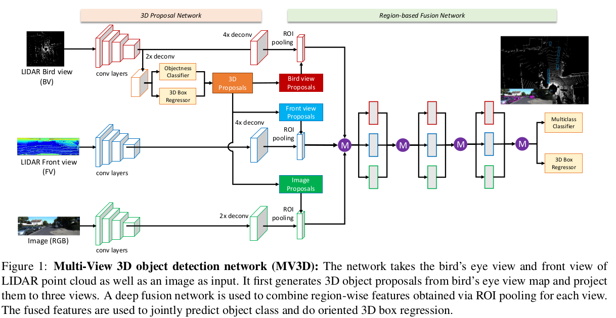
In the figure, the features of each view are converted by ROI pooling into feature vectors of the same size, then concatenated and finally fused further through Deep fusion.
Structural regularization
The network structure also uses two methods: drop-path and auxiliary losses.
In each iteration, a global drop path or a local drop path is chosen at random. For a global drop path, one of the three views is chosen at random, only the path on that view is kept and the paths of the other views are suppressed; for a local drop path, the path input to each connection node is randomly dropped with a probability of 50%.
The auxiliary losses structure is as follows:

This structure shares weights with the corresponding network layer and participates in the training loss backpropagation, and is removed at inference time.
Reference
Multi-View 3D Object Detection Network for Autonomous Driving