PointNet, PointNet++ and Frustum PointNet. The commonly used 3D point cloud object detection.
PointNet
PointNet applies deep learning directly to point cloud data. Point cloud data is a subset of the points in Euclidean space, and has three properties: disorder, the spatial relationship between points, and invariance.
- Disorder. Point cloud data is a set and is insensitive to the order of the data, which requires the model to be invariant to different permutations of the data. There are several approaches. The first is to sort the point cloud by some rule, but for high-dimensional space it is very hard to find a stable sorting rule. Another is to treat it as a sequence and train it with an RNN, but this approach struggles to handle input elements of extremely large length (thousands to tens of thousands, as in a point cloud). Finally the authors use a symmetric function to aggregate the information of each point: $f(\lbrace x_1,x_2,\cdots,x_n\rbrace)\approx g(h(x_1),h(h(x_2),\cdots,h(x_n))$, where the left side of the equation is the goal and the right side is the designed symmetric function. From this we can see that each point in the point cloud is processed separately with $h$ and then passed into the symmetric function $g$. In the paper the authors choose $h$ to be an MLP and $g$ to be max pooling.
- The spatial relationship between points. An object usually consists of point clouds in a specific space, and there are spatial relationships between points; PointNet exploits these relationships by concatenating global features with local features.
- Invariance. The object represented by point cloud data should be invariant to some spatial transformations (rigid transformations). PointNet aligns the point cloud data before extracting features to guarantee invariance. The alignment is achieved by training a small network (T-Net) to obtain a transformation matrix and multiplying it with the input point cloud data. This operation can be seen as adjusting the spatial points; intuitively it rotates them into an orientation that is favorable for classification or segmentation (a rigid transformation). In the actual implementation a related loss function is also added to make the transformation matrix approximately orthogonal, so as to reduce the loss of point cloud information. (Regularization: $L_{reg}=\lVert I-AA^T\rVert_F^2$, that is, an L2 loss)
The rough structure of PointNet is as follows:
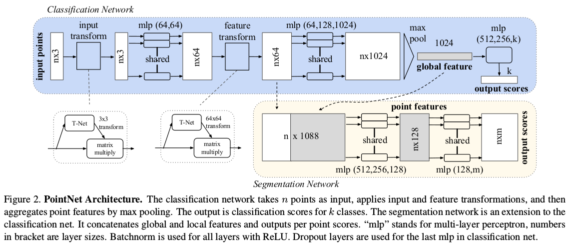
The figure contains both the classification and the segmentation part, where segmentation combines the global pooled feature with the point cloud features after the second alignment. In the source code the classification part uses T-Net while the segmentation part can do without it, with little improvement to the results, mainly because the PointNet structure itself cannot learn the local relationships between points, even with T-Net added.
PointNet++
PointNet++ improves on some of the problems of PointNet.
First let me introduce the basic network layers
- Sampling layer. Usually the raw point cloud data is enormous, and extracting local features for every point would be extremely expensive, so PoinNet++ samples the point cloud first. The sampling method used is Farthest Point Sampling (FPS), which covers the whole sampling space better than random sampling.
- Grouping layer. To obtain the local features of a point, we need to obtain the local region of that point. In images, the local region of a pixel is defined as the pixels within a certain Manhattan distance around it. For point cloud data, the local region of a point is defined as the points within a sphere of a given radius around it. The grouping layer finds the points contained in the local region formed around each sampled point, so that features can be extracted afterwards.
- Feature extraction layer. Here PointNet is borrowed to extract features from each local point cloud.
The layers above form the basic module of PointNet++. These basic modules are similar to those of a CNN; cascading several such modules gives PointNet++, which can extract shallow to deep features from point cloud data. The improvements over PointNet are as follows:
- PointNet only expresses the features of each point and has a poor ability to extract local structural information. So PointNet++ uses a sampling layer and a grouping layer to integrate local neighborhoods.
- PointNet’s global feature is obtained directly by max pooling, which causes a large information loss for both classification and segmentation tasks. For this reason PointNet++ downsamples level by level through multiple set abstractions (as shown below), obtaining local-global features of different scales and levels.
- For segmentation tasks, PointNet directly concatenates the global feature and the local feature, which produces weak discriminative features, whereas PointNet++ designs an encoder-decoder structure for classification and segmentation tasks; for the segmentation part, it first downsamples and then upsamples, using skip connections to concatenate the local-global features of the corresponding layers.
Finally the rough structure of the model is as follows:
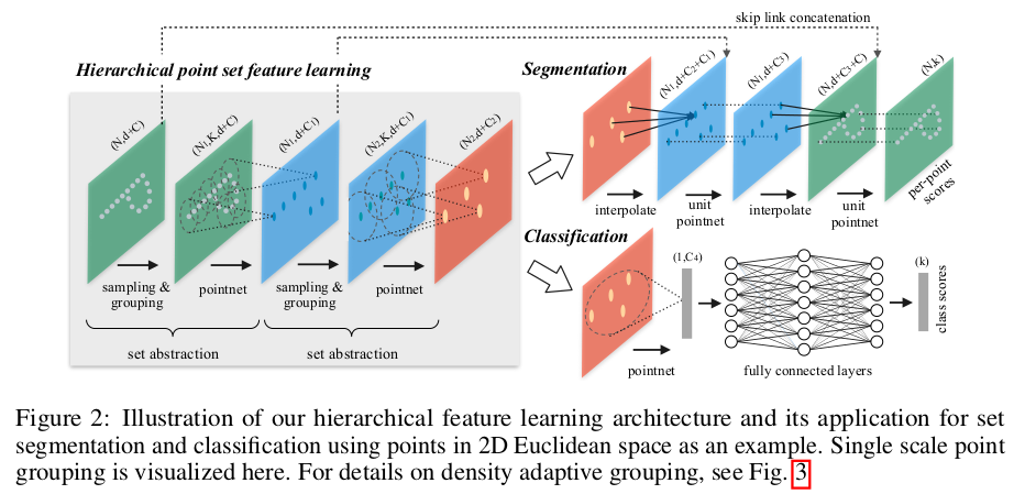
Since the distribution of a point cloud in space is irregular and non-uniform, although PointNet++ can learn the local features of a point cloud, the non-uniform distribution of the point cloud in each local region may prevent the model from extracting features well. For this reason the authors adopt two methods:
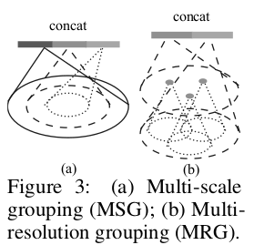
- Multi-Scale Grouping (MSG). That is, local features of different scales are extracted and concatenated together. This operation increases the computation considerably. As shown in figure a below
- Multi-Resolution Grouping (MRG). In this method the features extracted for each local region are represented by two concatenated vectors, as shown in figure b below. The first part is obtained by passing the features extracted by the previous layer through the feature extraction layer again, and the second part is obtained by directly extracting features from all the points in the raw point cloud data corresponding to this local region.
Principle of the FPS algorithm:
- The input point cloud has $N$ points; randomly choose one point $P_0$ as the starting point, giving the sample set $S=\lbrace P_0\rbrace$;
- Compute the distance from every point to $P_0$, forming an $N$-dimensional array $L$, choose the point with the largest distance as the sampling point $P_1$ and add it to the sample set $S=\lbrace P_0,P_1\rbrace$;
- Compute the distance from every point to $P_1$; for each point $N_i$, if its distance to $P_1$ is smaller than $L[i]$, update the distance array $L[i]=d(N_i,P_1)$, that is, the array $L$ stores the nearest distance from each point to the sample set $S$;
- Select the point corresponding to the maximum value in $L$ and add it to the sample set $S=\lbrace P_0,P_1,P_2\rbrace$;
- Repeat steps 2-4 until the length of the sample set reaches $n$, that is, $n$ target points have been sampled
This involves the choice of the initial point and the distance metric, generally as follows:
- Choice of the initial point:
- Pick a random point, so that the result differs every time
- Pick the point farthest from the centroid of the point cloud, so that the result is the same every time and the initial point is usually located at a local extremum, with a certain descriptive ability
- Distance metric:
- Euclidean distance, mainly for point clouds, giving uniform sampling in 3D space
- Geodesic distance, that is, the distance of the shortest path between two vertices along the mesh surface, mainly for triangle meshes, giving uniform sampling over the triangle mesh surface
Finally let me mention the decoder of the segmentation task. After the processing of the encoder above, what we have is the feature representation of a small number of points; to segment the point cloud, PointNet++ uses a form of inverse interpolation to upsample. Specifically:
Suppose the point cloud before interpolation is $P_1$ with dimension $N_1\times C$, and the point cloud after it is $P_2$ with dimension $N_2\times C_2$, where $N_2\gt N_1$ (since this operation is upsampling). The upsampling computation follows the formula below:
$$ \begin{aligned} & f^{(j)}(x)=\frac{\sum_{i=1}^kw_i(x)f_i^{(j)}}{\sum_{i=1}^kw_i(x)} \\ where\qquad &w_i(x)=\frac{1}{d(x,x_i)^p}, \ j=1,2,\cdots,C \end{aligned} $$That is, for each point $x$ in $P_2$, find the $k$ points $x_1,x_2,\cdots,x_k$ in the point cloud space $P_1$ before sampling that are closest to it, and the weighted sum of the features of these $k$ points gives the feature of $x$, where the weight is inversely related to the distance, that is, the farther away, the lower the contribution. The distance metric function here is $d$. The parameters chosen in the paper are $p=2$ and $k=3$.
The operation above only gives global-level features; to obtain accurate segmentation results we also need local-level features, so PointNet++ adds skip connections. The operation is fairly simple: take the point cloud features of the corresponding encoder layer, concatenate them with the current layer, and then integrate them through a unit pointnet (a series of MLPs). For details, refer to the PointNet++ network structure figure above.
Frustum PointNet
Detection by combining RGB image information with point cloud information. The main pipeline is: first obtain the object boxes in the 2D image through an object detection model, map the object boxes into the 3D point cloud to obtain frustum proposals, and then use a point cloud based model to perform instance segmentation and 3D bounding box regression on the frustum proposal regions. The rough structure is as follows:
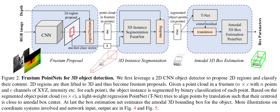
The first part in the figure is the 2D object detection network, which gives the object boxes and their classes; the object boxes are then mapped to 3D frustum proposals. The second part is the instance segmentation part: the points in the frustum proposal obtained in the previous part are sampled to $N$ points with dimension $N\times C$, and together with the previously obtained one-hot class vector they are used as the input of the instance segmentation network, which outputs a mask. In the last part, the $M$ points filtered by the mask from the previous step are used as input, first corrected and aligned by T-Net, and then another network regresses and predicts the 3D bounding box.
When mapping the 2D detection boxes into the 3D point cloud to generate frustum proposals, since each frustum proposal has a different orientation, the paper rotates it to be orthogonal to the camera, which increases the rotation invariance of the subsequent algorithm. As shown from a to b below.

When only the frustum proposal is used, the resulting point cloud contains a large number of background points. So the instance segmentation in the second part separates the foreground from the background, and the segmented foreground points are also centered to introduce translation invariance, as shown in figure c above.
Although the instance segmentation part obtains the center point of the object, the foreground point cloud may not fully contain the object, so the center point still needs to be corrected. The last part uses T-Net to learn the residual of the object center point. Finally Box Estimation Net outputs the various parameters of the final 3D bounding box, with an output dimension of $3+4\times NS+2\times NH$, where 3 represents the residual regression for the center point (XYZ), attached after the T-Net regression; $NS$ represents the number of anchors of different sizes, each anchor having four dimensions, namely the confidence of that anchor and the residual regression of length, width and height; $NH$ represents the anchors of different orientations, each anchor having two parameters, namely the confidence and the orientation angle $\theta$.
The detailed structure of the parts of the model after the 2D detection network is roughly as follows: (two versions are included, corresponding to using PointNet and PointNet++ to extract point cloud features)
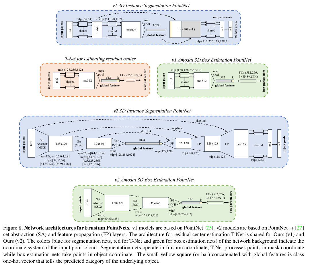
In practice the size and angle of a 3D bounding box jointly determine the box information, so the paper also proposes a corner loss for the bounding box:
$$ L_{corner} = \sum_{i=1}^{NS}\sum_{j=1}^{NH}\delta_{ij}min\{\sum_{k=1}^8\vert\vert P_k^{ij}-P_k^\ast\vert\vert, \sum_{i=1}^8\vert\vert P_k^{ij}-P_k^{\ast\ast}\vert\vert\} $$Among the $NS\times NH$ anchors, only the bounding box with the correct size and head orientation incurs the loss (in the remaining cases $\delta=0$). For the $k$-th corner $P_k^{ij}$ of the box with the $i$-th size and the $j$-th orientation, it is moved to the center of the ground truth box and the L1 loss is computed with each corresponding corner. Considering the 180-degree flip problem, the loss with the corner after a 180-degree rotation, $P^{\ast\ast}$, is also computed and the minimum is taken. The overall loss is as follows:
$$ L_{multi−task} =L_{seg} + \lambda(L_{c1−reg} + L_{c2−reg} + L_{h−cls} + L_{h−reg} + L_{s−cls} + L_{s−reg} + \gamma L_{corner}) $$Reference
PointNet: Deep Learning on Point Sets for 3D Classification and Segmentation
PointNet++: Deep Hierarchical Feature Learning on Point Sets in a Metric Space
Frustum PointNets for 3D Object Detection from RGB-D Data