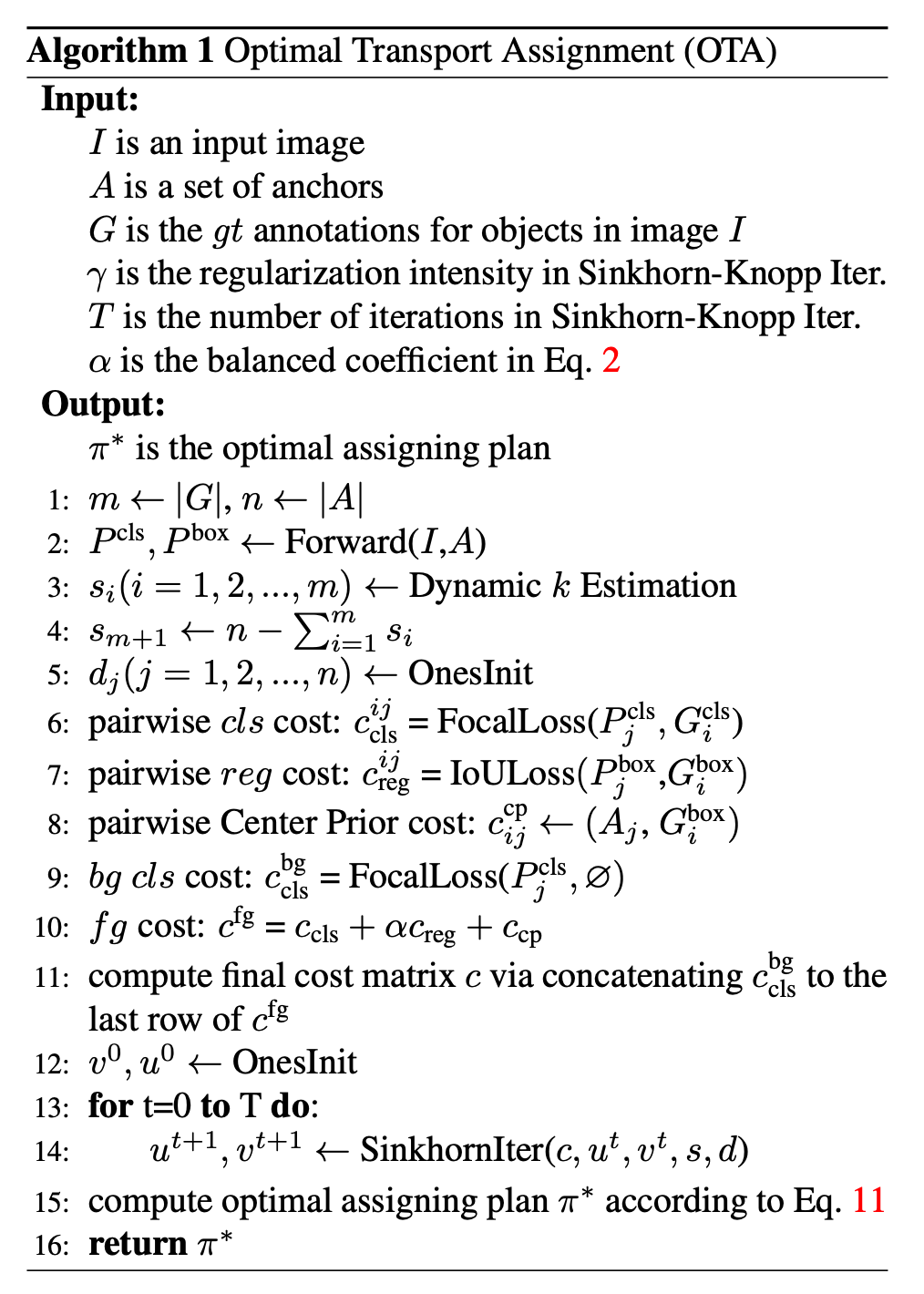
Deciding which gt to assign to which anchor is an important problem in object detection, namely the label assignment problem. OTA offers a new angle on this problem: treating label assignment as an optimal transport problem.
Label Assignment
Previous label assignment strategies are mainly divided into two kinds: fixed and dynamic.
For fixed label assignment, Anchor-based detection models usually use an IoU threshold as the assignment criterion (such as Fast-RCNN, Faster-RCNN, YoLo3, RetinaNet and so on), while some Anchor-free detection models designate anchors within a certain range of the object center as positive samples (such as FCOS, Foveabox and so on). Fixed assignment methods usually adopt a fixed assignment strategy (for example a fixed IoU threshold or a fixed radius), which is the same for objects of different sizes and shapes, so the model may end up with a suboptimal assignment.
For dynamic label assignment, the prediction confidence of each anchor is generally used as a dynamic assignment criterion, and anchors with high confidence are assigned to the relevant objects; however, dynamic assignment methods can still suffer from ambiguous anchor assignment because they cannot exploit global information.
OTA exploits global information and views label assignment as an optimal transport problem, with the main goal of finding the globally optimal matching of the objects in the image.
Optimal Transport
The standard optimal transport problem is as follows:
There are $m$ suppliers and $n$ demanders. The $i$th supplier can provide $s_i$ goods, and the $j$th demander needs $d_j$ goods. The cost of transporting one unit of goods from supplier $i$ to demander $j$ is defined as $c_{ij}$. The goal of the OT problem is to find a transport plan $\pi^\ast=\{\pi_{i,j}\vert i=1,2,\dots,m, j=1,2,\dots,n\}$ that minimizes the cost of transporting all goods, expressed as follows:
$$ \begin{aligned} \min_{\pi}& \sum_{i=1}^m\sum_{j=1}^n c_{ij}\pi_{ij} \\ s.t. & \sum_{i=1}^m\pi_{ij} = d_j,\quad \sum_{j=1}^n\pi_{ij} = s_i \\ & \sum_{i=1}^ms_i = \sum_{j=1}^nd_j \\ & \pi_{ij} \ge 0,\quad i=1,2,\dots,m,\quad j=1,2,\dots,n \end{aligned} $$This problem can be solved in linear time, but considering the feature map dimensions and anchor scales involved in object detection, the authors use Sinkhorn Iteration to deal with the excessive computation time.
Sinkhorn Iteration converts the linear programming problem above into the following convex nonlinear form with an added entropy regularization term:
$$ \min_\pi \sum_{i=1}^m\sum_{j=1}^n c_{ij}\pi_{ij}+\gamma E(\pi_{ij}) $$where $E(\pi_{ij}) = \pi_{ij}(\log\pi_{ij}+1)$ and $\gamma$ is a hyperparameter controlling the strength of the regularization. By the Lagrange multiplier method we have:
$$ \min_\pi \sum_{i=1}^m\sum_{j=1}^n c_{ij}\pi_{ij}+\gamma E(\pi_{ij})+\alpha_j(\sum_{i=1}^m\pi_{ij}-d_j)+\beta_i(\sum_{j=1}^n\pi_{ij}-s_i) $$where $\alpha_j(j=1,2,\dots,n)$ and $\beta_i(i=1,2,\dots,m)$ are the Lagrange multipliers. Taking the derivative of the formula above and setting it to 0 gives:
$$ \pi_{ij}^\ast = \exp(-\frac{\alpha_j}{\gamma})\exp(-\frac{c_{ij}}{\gamma})\exp(-\frac{\beta_i}{\gamma}) $$Let $u_j = \exp(-\frac{\alpha_j}{\gamma})$, $v_i = \exp(-\frac{\beta_i}{\gamma})$ and $M_{ij} = \exp(-\frac{c_{ij}}{\gamma})$. Then the constraints can be rewritten as:
$$ \begin{aligned} \sum_i\pi_{ij} &= u_j(\sum_iM_{ij}v_i) = d_j \\ \sum_j\pi_{ij} &= (\sum_ju_jM_{ij})v_i = s_i \end{aligned} $$The two equations above must hold simultaneously, which gives the following iterative update:
$$ \begin{aligned} u^{t+1}_j &= \frac{d_j}{\sum_iM_{ij}v^t_i} \\ v^{t+1}_i &= \frac{s_i}{\sum_jM_{ij}u^{t+1}_j} \end{aligned} $$After $T$ iterations, the optimal plan $\pi^\ast$ is computed as follows:
$$ \pi^\ast = diag(v)Mdiag(u) $$In the paper the authors set $\gamma=0.1$ and $T=50$.
Optimal Transport for Label Assignment
Combining the label assignment problem with the OT problem: the authors treat gt as suppliers, with each gt supplying $k$ labels ($s_i=k,i=1,2,\dots,m$), and anchors as demanders, with each anchor needing 1 label (that is, $d_j=1,j=1,2,\dots,n$). The transport cost of one positive label from a gt to an anchor is defined as $c^{fg}$, taken as the sum of the $cls$ and $reg$ losses:
$$ c^{fg}_{ij} = L_{cls}(P^{cls}_{ij}(\theta),G^{cls}_i)+\alpha L_{reg}(P^{box}_j(\theta),G^{box}_i) $$where $\theta$ denotes the model parameters, $P^{cls}_j$ and $P^{box}_j$ denote the predicted $cls$ score and box coordinates produced by anchor $a_j$, and $G^{cls}_i$ and $G^{box}_i$ denote the class and box coordinates of the ground truth annotation $gt_i$. $L_{cls}$ and $L_{reg}$ are the classification loss (cross-entropy loss or Focal loss can be used) and the box regression loss (IoU loss, GIoU loss or SmoothL1 loss can be used). $\alpha$ is a balancing factor.
Besides the matching of positive samples, a considerable portion of anchors are designated as negative samples during training, so the authors also add negative sample assignment by introducing a background supplier (which only provides negative labels). In the standard OT problem the total supply of the suppliers should equal the total demand of the demanders, so the background supply is computed as follows:
$$ c^{bg}_j =L_{cls}(P^{cls}_j(\theta), \varnothing) $$where $\varnothing$ denotes the background class. Appending $c^{bg}\in R^{1\times n}$ to the end of $c^{fg}\in R^{m\times n}$ gives the complete cost matrix $c\in R^{(m+1)\times n}$, and the supply vector $s$ is updated accordingly as follows:
$$ s_i = \begin{cases} k, & if\quad i\le m \\ n-m\times k, & if\quad i=m+1 \end{cases} $$Given the cost matrix $c$, the supply vector $s\in R^{m+1}$ and the demand vector $d\in R^n$, solving this OT problem gives the optimal assignment plan $\pi^\ast\in R^{(m+1)\times n}$.
Some optimization designs
- Center prior. That is, anchors are selected for assignment within a designated region around the object center. In theory OTA can designate any anchor in the global scope as a positive sample, and the center prior lets OTA focus more on the potential positive sample regions, which stabilizes the early training of the model. The concrete operation used by the authors is: for each gt, select the top $r^2$ anchors in each FPN layer according to the center distance between the anchor and the gt as positive sample candidates; for the remaining anchors that are not selected, a constant is added at the corresponding position of the cost matrix to reduce the probability of the anchor being selected as a positive sample.
- Dynamic $k$ estimation. Generally each gt should have a different suitable number of positive anchors/points, because each gt has a different size, scale and degree of occlusion. Based on the IoU values between the predicted boxes and the gt, the authors select the top q IoU values for each gt and take their sum as the suitable number of positive anchors/points for that gt (because the suitable number of positive anchors/points for a gt should be positively correlated with the number of anchors/points that can regress that gt well).
Putting the above together, the pseudo-code of OTA is as follows: