A lightweight stereo matching module is introduced into the 2D real-time object detection framework yolo to achieve efficient 3D object detection. The rough structure is shown below:
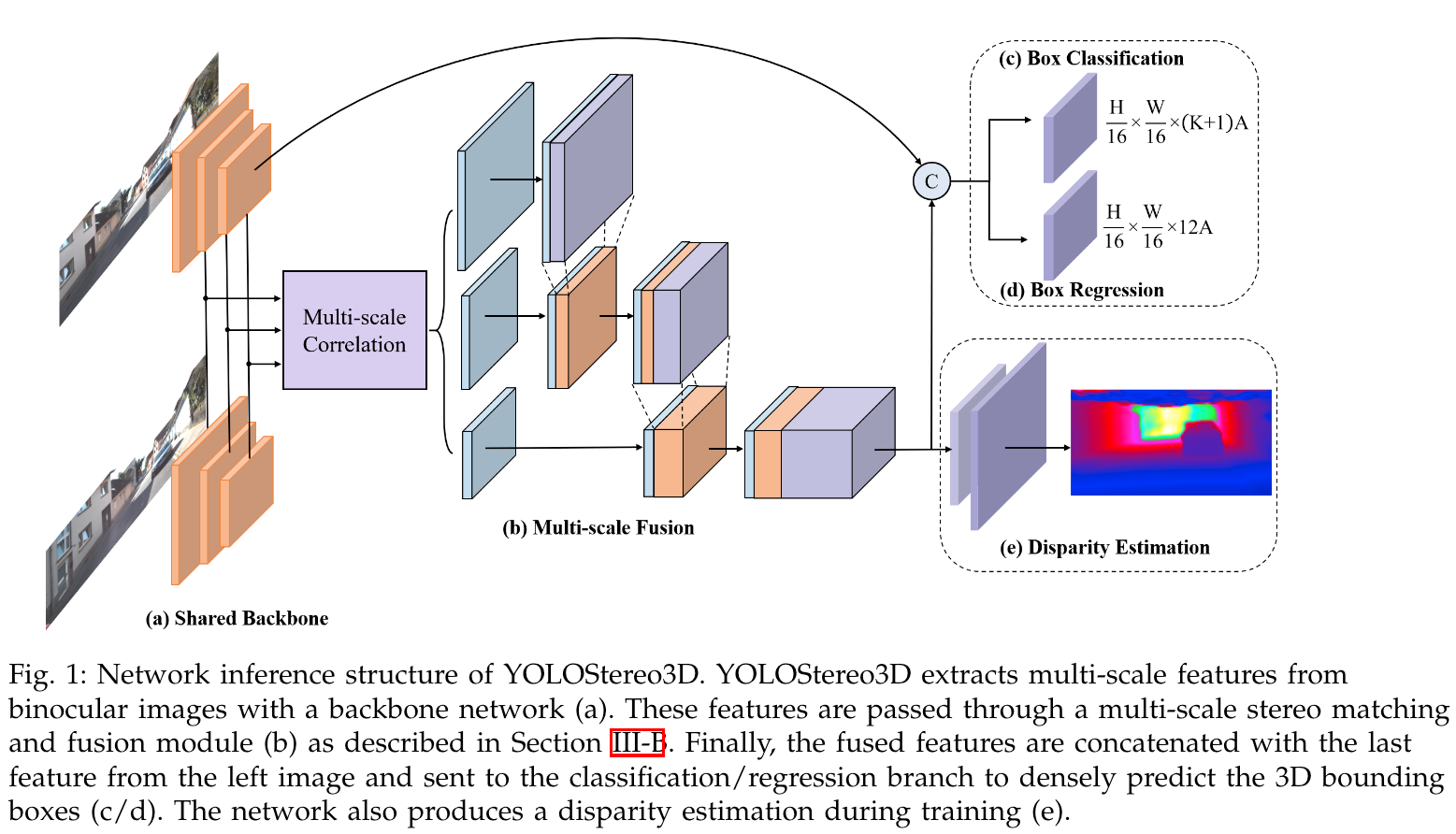
Anchors
For 3D object detection, the original yolo anchors designed for 2D objects need to be redesigned. The authors use 12 parameters to represent an anchor:
- $[x_{2d}, y_{2d}, w_{2d}, h_{2d}]$, representing the 2D object box
- $[c_x, c_y, z]$ represents the position of the 3D object center in the left image
- $[w_{3d}, h_{3d}, l_{3d}]$ represents the width, height and length of the 3D object box
- $[sin(2\alpha), cos(2\alpha)]$ to estimate the angle of the object
Here the authors found that $[sin\alpha, cos\alpha]$ and $[sin(\alpha+\pi), cos(\alpha+\pi)]$ may produce identical rectangular boxes, so they use $[sin(2\alpha), cos(2\alpha)]$ to represent the angle of the object, and additionally add a classification branch to predict whether $\vert\alpha\vert \gt \frac{\pi}{2}$, which also indicates whether the object is facing the camera.
A 3D statistical prior is applied to the anchors to improve the regression results. Iterating over the training set, for each anchor of a different size, the object boxes assigned to that anchor are collected based on IOU, and then the averages of $z$, $sin(2\alpha)$ and $cos(2\alpha)$ are computed. Because 3D boxes of different classes differ considerably, the authors collect the 3D prior information per class.
Considering the application scenario of autonomous driving, the authors project each anchor back into 3D space according to its average $z$ value, and then filter out the anchors that are far from the ground. This filtering is also done per class.
Multi-Scale Stereo Feature Extraction
For stereo matching, the main task is to build a cost volume. The current best method is the concatenation-based approach: the right feature map is shifted horizontally over the left feature map to compute the cost volume. To reduce computation time, the authors adopt a correlation-based method to build a lightweight cost volume: a normalized dot-product layer is used to compute over the left and right feature maps (see the inner-product layer and correlation layer mentioned in the two papers cited there). The output dimension of this method is $[B, max\_disp, H, W]$; the number of output channels is small, which makes the model’s fusion stage lean towards monocular features, and subsequent downsampling of the result loses further information.
The authors use a ghost module to expand the number of channels. The ghost module uses depthwise convolution to produce additional features. The authors go further and concatenate the output of the ghost module with the input, tripling the number of channels. In part b of the structure figure above, the light purple part is the output of the ghost module.
To minimize information loss in the stereo matching stage while keeping computation time under control, the authors build a hierarchical multi-scale fusion mechanism:
At downsampling rates of 4x and 8x, the authors build cost volumes with a maximum disparity of 96 and 192 respectively, which are then fed into the ghost module, downsampled and concatenated with later, smaller-scale feature maps. At a downsampling rate of 16x, the number of channels is first downsampled with a $1\times 1$ convolution, and then the authors use the concatenation-based method to create a small cost volume so as to retain more semantic information. The details are shown in the structure figure above.
Training Scheme and Loss Function
First, for data augmentation, the authors apply photometric distortion to both stereo images simultaneously and perform random flipping during training. The random flipping here includes flipping the RGB images together, flipping the position and direction of the objects, and then swapping the left and right images.
As can be seen from the structure figure, the model has an extra auxiliary branch during training. Disparity supervision is important for improving the detection performance of the model. The authors upsample the final stereo feature to $[W/4, H/4]$, and supervise the predicted disparity with a coarse disparity ground truth obtained by the traditional block matching algorithm in OpenCV. At inference time this branch is not involved in the computation.
As for the loss function, focal loss is used for classification, smoothed-L1 loss for the object boxes, and stereo focal loss for the auxiliary disparity estimation (see AcfNet for details).
First the expected disparity distribution is computed (with the variance directly set to $\sigma = 0.5$):
$$ P(d) = softmax(-\frac{\vert d-d^{gt}\vert}{\sigma}) = \frac{exp(-c_d^{gt})}{\sum_{d'=0}^{D-1}exp(-c_{d'}^{gt})} $$where $d$ denotes the disparity and $c_d$ denotes the confidence when the predicted disparity is $d$. Then the stereo focal loss can be defined as:
$$ \mathcal{L}_{SF} = \frac{1}{\vert \mathcal{P}\vert}\sum_{p\in\mathcal{P}}\left(\sum_{d=0}^{D-1}(1-P_p(d))^{-\alpha}\cdot\big(-P_p(d)\cdot log\hat{P}_p(d)\big)\right) $$where $D$ is the defined maximum disparity (max-disparity), $\alpha$ is the weight of the focal loss (the larger $\alpha$ is, the higher the weight of the correct disparity value), $\mathcal{P}$ is the set of pixels involved in the computation, and $P_p(d)$ and $\hat{P}_p(d)$ denote the expected and the actually predicted disparity distribution functions, respectively.
The final loss function is defined as the sum of the three loss functions above.
Reference
YOLOStereo3D: A Step Back to 2D for Efficient Stereo 3D Detection