Monocular 3D detection is an important and challenging task in the autonomous driving field; the current difficulty is how to accurately predict the depth of objects. MonoRCNN uses geometric relations to decouple the depth estimation problem into the object’s real height and its projected height in the image.
The authors impose two conditions on the use of this model:
- The model only predicts the heading angle of the object, that is, the yaw angle
- The camera intrinsics are known during both training and inference
Architecture
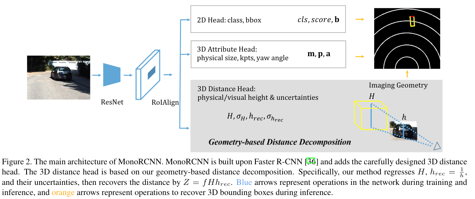
The model is similar to Faster R-CNN; the backbone is a combination of ResNet-50 and FPN, then RoIAlign is used to extract object features, followed by three branches: a 2D head, a 3D attribute head and a 3D distance head. The final predictions give the following parameters:
- class label $cls$ and confidence $score$
- 2D bounding box $\mathbf{b} = (x_1, y_1, x_2, y_2)$, represented by the top-left and bottom-right coordinates
- projected coordinates of the center point of the 3D bounding box in the image, $\mathbf{p} = (p_1, p_2)$
- physical size of the 3D bounding box $\mathbf{m} = (W, H, L)$, denoting the real width, height and length of the object respectively
- yaw angle of the 3D bounding box $\mathbf{a} = (sin\theta, cos\theta)$
- depth $Z$ of the center point of the 3D bounding box
MonoRCNN predicts the coordinates of the 3D bounding box center in the image coordinate system $(p_1, p_2, Z)$, which are then converted to a point in camera coordinates with the camera intrinsic matrix $\mathbf{P}$:
$$ \begin{bmatrix} p_1 \cdot Z \\ p_2 \cdot Z \\ Z \end{bmatrix}_P = \mathbf{P} \cdot \begin{bmatrix} x \\ y \\ z \\ 1 \end{bmatrix}_C $$3D Distance Head
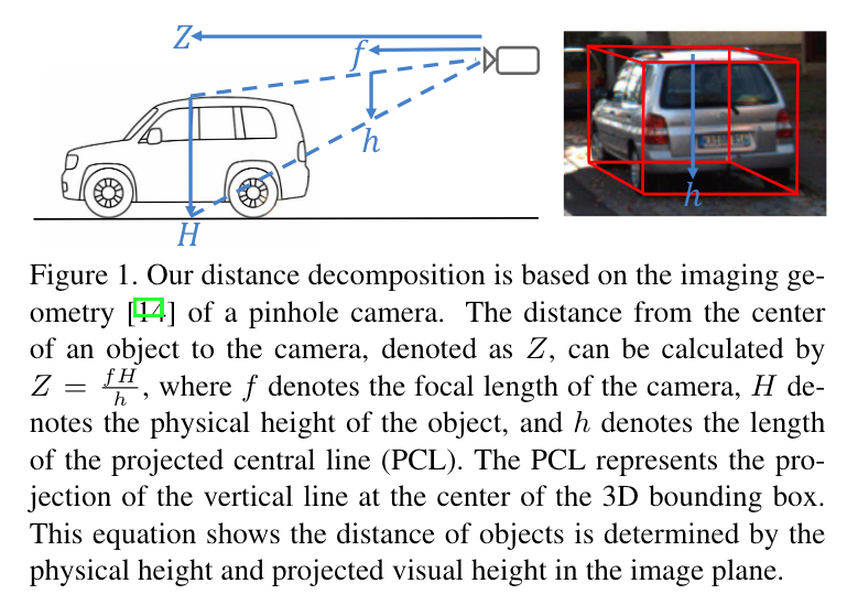
As shown above, from simple geometric relations we obtain:
$$ Z = \frac{fH}{h} = fHh_{rec} $$where $h_{rec} = \frac{1}{h}$. The authors predict $H$ and $h_{rec}$ by regression to obtain $Z$ indirectly. Since only the object height in the image needs to be obtained, this method can effectively deal with complex scenarios such as occlusion, reflection and truncated objects. At the same time, this decoupling also maintains self-consistency, so that depth can still be predicted accurately even when both predicted heights are inaccurate: for example, when the predicted $H$ is larger, the model adaptively decreases $h_{rec}$. For the details of this part, refer to the original paper.
The loss function of this branch is an uncertainty-aware regression loss:
$$ \begin{aligned} L_H &= \frac{L_1(\hat{H}, H)}{\sigma_H} + \lambda_Hlog(\sigma_H) \\ L_{h_{rec}} &= \frac{L_1(\hat{h}_{rec}, h_{rec})}{\sigma_{h_{rec}}} + \lambda_{h_{rec}}log(\sigma_{h_{rec}}) \end{aligned} $$where $\hat{H}$ and $\hat{h}_{rec}$ are the ground truths, $H$ and $h_{rec}$ are the predictions, $\lambda_H$ and $\lambda_{h_{rec}}$ are positive coefficients used to balance the uncertainty terms, and $\sigma_H$ and $\sigma_{h_{rec}}$ are learnable variables for the uncertainty.
The authors show experimentally that $\sigma_{h_{rec}}$ is more discriminative for objects at different distances than $\sigma_H$, and that $fH\sigma_{h_{rec}}$ can represent the uncertainty of the distance. So the authors use $\frac{score}{fH\sigma_{h_{rec}}}$ instead of $score$ to rank the predictions in order to improve model accuracy.
3D Attribute Head
This branch mainly predicts the physical size of the object, the yaw angle and the 2D keypoints. For the physical size and yaw angle, an L1 loss is used directly for regression:
$$ \begin{aligned} L_{size} &= L_1(\hat{\mathbf{m}}, \mathbf{m}) \\ L_{yaw} &= L_1(\hat{\mathbf{a}}, \mathbf{a}) \end{aligned} $$For the 2D keypoints, define: $\hat{\mathbf{t}} = \left ( \frac{\hat{p}_1 - x_1}{x_2 - x_1}, \frac{\hat{p}_2 - y_1}{y_2 - y_1} \right )$, then:
$$ L_{kpt} = L_1(\hat{\mathbf{t}}, \mathbf{t}) $$Finally, the overall loss of the model is as follows:
$$ \begin{aligned} L =& \lambda_{cls}L_{cls} + \lambda_{bbox}L_{bbox} + \lambda_{size}L_{size} \\ &+ \lambda_{yaw}L_{yaw} + \lambda_{kpt}L_{kpt} + \lambda_HL_H + \lambda_{h_{rec}}L_{h_{rec}} \end{aligned} $$where $\lambda_{cls}=1$, $\lambda_{bbox}=1$, $\lambda_{size}=3$, $\lambda_{yaw}=5$, $\lambda_{kpt}=5$, $\lambda_{H}=0.25$, $\lambda_{h_{rec}}=1$
Reference
Geometry-based Distance Decomposition for Monocular 3D Object Detection