Normally the pixel values of an image are discrete (between 0 and 255), so we can actually regard an image as a sequence of length $H\times W\times C$. When predicting the current pixel value, the preceding pixel values are taken as known information and participate in the prediction, and this proceeds recursively pixel by pixel, which is the autoregressive model:
$$ p(x) = p(x_1)p(x_2\vert x_1)\dots p(x_n\vert x_1,x_2,\dots,x_{n-1}) $$But the process above generates one pixel at a time, so it runs slowly. VQ-VAE borrows the idea of the autoregressive model, and its most obvious characteristic is that the latent variable obtained through the encoder is a discrete variable, which compresses the image into a small feature space. The overall pipeline is roughly shown below:
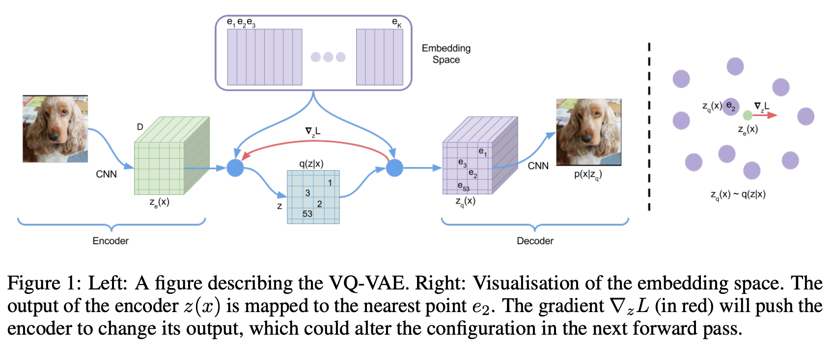
- The input $\mathbf{x}$ of size $H\times W\times 3$ is passed through the encoder to obtain a preliminary intermediate variable $\mathbf{z}=\text{encoder}(\mathbf{x})$ of reduced size $h\times w\times d$
- The model maintains an embedding layer $\mathbf{E}=[\mathbf{e}_1, \mathbf{e}_2, \dots, \mathbf{e}_K]$, that is, the codebook, where each $\mathbf{e}_i$ has length $d$. For each $d$-dimensional vector in $\mathbf{z}$, nearest neighbor search gives the corresponding $\mathbf{e}_i$ value, that is, the mapping $\mathbf{z}_q(\mathbf{x}) =\mathbf{e}_{argmin_j\vert\vert \mathbf{z}(\mathbf{x})-\mathbf{e}_j\vert\vert_2}$. The resulting encoding vector is denoted $\mathbf{z}_q$, and such an encoding vector is in fact a discrete vector
- $\mathbf{z}_q$ is fed into the decoder to obtain the result $\hat{\mathbf{x}} = \text{decoder}(\mathbf{z}_q)$
The paper gives the loss function of VQ-VAE as follows:
$$ L = -\log p(\mathbf{x}\vert\mathbf{z}_q(\mathbf{x}))+\vert\vert\text{sg}[\mathbf{z}(\mathbf{x})]-\mathbf{z}_q(\mathbf{x})\vert\vert_2^2+\beta\vert\vert\mathbf{z}(\mathbf{x})-\text{sg}[\mathbf{z}_q(\mathbf{x})]\vert\vert_2^2 $$The first term is used to optimize the encoder and the decoder, that is, the reconstruction loss; from the figure we can also see that the gradient of the loss with respect to $\mathbf{z}$ is passed to the encoder. This term is usually the MSE loss between the reconstructed image and the input image, $\vert\vert \mathbf{x}-\text{decoder}(\mathbf{z}_q)\vert\vert_2^2$.
Because our forward computation involves the $\argmin$ operation, which has no gradient, the authors use the Straight-Through Estimator method to artificially design a gradient, namely $\vert\vert \mathbf{x}-\text{decoder}(\mathbf{z} + \text{sg}[\mathbf{z}_q-\mathbf{z}])\vert\vert_2^2$. The $\text{sg}$ in the formula stands for stop gradient, that is, it is 0 during backpropagation and the original value in the forward computation, described mathematically as follows:
$$ \text{sg}(x) = \begin{cases} x \quad \text{in forward process} \\ 0 \quad \text{backward process} \end{cases} $$The last two terms of the loss function are related to the codebook. Usually we want $\mathbf{z}_q$ and $\mathbf{z}$ to be as close as possible, so the optimization objective is $\vert\vert\mathbf{z}_q - \mathbf{z}\vert\vert_2^2$. Since the gradient of this objective equals the gradient with respect to $\mathbf{z}$ plus the gradient with respect to $\mathbf{z}_q$, we can equivalently write it as follows:
$$ \vert\vert\text{sg}[\mathbf{z}]-\mathbf{z}_q\vert\vert_2^2 + \vert\vert\mathbf{z}-\text{sg}[\mathbf{z}_q]\vert\vert_2^2 $$Equivalent here means the gradients are equivalent; the loss value actually computed in the forward pass is twice the original. In the formula above, the first term is the gradient of $\mathbf{z}_q$, which amounts to fixing $\mathbf{z}$ and moving $\mathbf{z}_q$ towards $\mathbf{z}$; the second term is the gradient of $\mathbf{z}$, which amounts to fixing $\mathbf{z}_q$ and moving $\mathbf{z}$ towards $\mathbf{z}_q$. Since $\mathbf{z}_q$ is freer than $\mathbf{z}$ (as $\mathbf{z}$ is the output of the encoder), and to do our best to guarantee the reconstruction quality, we should try to make $\mathbf{z}_q$ approach $\mathbf{z}$. This step can use weights to adjust the importance of each loss term.
In summary, the final loss function of VQ-VAE is as follows:
$$ L = \vert\vert \mathbf{x}-\text{decoder}(\mathbf{z} + \text{sg}[\mathbf{z}_q-\mathbf{z}])\vert\vert_2^2 + \gamma\vert\vert\text{sg}[\mathbf{z}]-\mathbf{z}_q\vert\vert_2^2 +\beta \vert\vert\mathbf{z}-\text{sg}[\mathbf{z}_q]\vert\vert_2^2 $$where $\beta \lt \gamma$; the paper chooses $\gamma = 1$ and $\beta = 0.25$.
From the description above we can see that VQ-VAE actually has little to do with VAE; it is merely an AE model whose goal is image reconstruction.
In the VQ-VAE paper, the authors use PixelCNN to predict $\mathbf{z}_q$, which enables random image generation. During training the model trains VQ-VAE and PixelCNN jointly: the input data is passed through the encoder to obtain $\mathbf{z}$, the codebook is queried to obtain $\mathbf{z}_q$, and then PixelCNN produces a variable $\mathbf{z}_p$ of the same size as $\mathbf{z}_q$, which serves as the input of the decoder. At inference time, by contrast, an empty image is fed directly into PixelCNN to obtain $\mathbf{z}_p^\prime$, which is then fed directly into the decoder to generate an image.
For the PixelCNN model, see this article.