Note: VAE is not a model that only cares about reconstruction; its more important ability is image generation, so VAE is not an AE model — it has generative ability.
Unlike the common Autoencoder, the variational autoencoder does not map the input to a fixed vector but to a distribution $p_\theta$ (with parameters $\theta$). The relationship between the input data $\mathbf{x}$ and the latent variable $\mathbf{z}$ is as follows:
- $p_\theta(\mathbf{z})$: prior probability
- $p_\theta(\mathbf{x}\vert\mathbf{z})$: likelihood
- $p_\theta(\mathbf{z}\vert\mathbf{x})$: posterior probability
Assuming that after obtaining the optimal model parameters $\theta^{\star}$ we can generate samples that follow the real data distribution through the following steps:
- Sample a $\mathbf{z}^{(i)}$ from the prior $p_{\theta^\star}(\mathbf{z})$
- Generate $\mathbf{x}^{(i)}$ according to the conditional probability $p_{\theta^\star}(\mathbf{x}\vert\mathbf{z}=\mathbf{z}^{(i)})$
The optimal parameters $\theta^\star$ can be obtained by maximizing the probability of recovering the real data distribution:
$$ \theta^\star = argmax_\theta\prod_{i=1}^np_\theta(\mathbf{x}^{(i)}) $$Moving to log space gives:
$$ \theta^\star = argmax_\theta\sum\log p_\theta(\mathbf{x}^{(i)}) $$To bring in an encoding vector we have:
$$ p_\theta(\mathbf{x}^{(i)}) = \int p_\theta(\mathbf{x^{(i)}}\vert\mathbf{z})p_\theta(\mathbf{z})d\mathbf{z} $$According to the formula above, we would need to iterate over all $\mathbf{z}$ to compute it, so in practice $p_\theta(\mathbf{x}^{(i)})$ is very hard to obtain. The authors solve this problem with an approximate distribution, that is, for each input sample $\mathbf{x}$, a distribution $q_\phi(\mathbf{z}\vert\mathbf{x})$ parameterized by $\phi$ is introduced to directly approximate the posterior distribution $p_\theta(\mathbf{z}\vert\mathbf{x})$. This guarantees a one-to-one correspondence between the input sample, the latent variable and the reconstructed sample. So the final structure of VAE is fairly similar to that of an Autoencoder:
- The latent variable is obtained from the approximate posterior $q_\phi(\mathbf{z}\vert\mathbf{x})$, that is, the encoder part. $q_\phi(\mathbf{z}\vert\mathbf{x})$ is also called the probabilistic encoder.
- The result is generated from the likelihood $p_\theta(\mathbf{x}\vert\mathbf{z})$, which corresponds to the decoder part. $p_\theta(\mathbf{x}\vert\mathbf{z})$ is also called the probabilistic decoder.
We want the approximate distribution $q_\phi(\mathbf{z}\vert\mathbf{x})$ to be as similar as possible to $p_\theta(\mathbf{z}\vert\mathbf{x})$. A natural idea is to minimize the KL divergence between them, $D_{KL}(q_\phi(\mathbf{z}\vert\mathbf{x})\vert\vert p_\theta(\mathbf{z}\vert\mathbf{x}))$. Expanding and simplifying $D_{KL}$ gives:
$$ \begin{aligned} & D_\text{KL}( q_\phi(\mathbf{z}\vert\mathbf{x}) \vert\vert p_\theta(\mathbf{z}\vert\mathbf{x}) ) \\ =& \log p_\theta(\mathbf{x}) + D_\text{KL}(q_\phi(\mathbf{z}\vert\mathbf{x}) \vert\vert p_\theta(\mathbf{z})) - \mathbb{E}_{\mathbf{z}\sim q_\phi(\mathbf{z}\vert\mathbf{x})}\log p_\theta(\mathbf{x}\vert\mathbf{z}) \end{aligned} $$that is:
$$ \begin{aligned} & \log p_\theta(\mathbf{x}) - D_\text{KL}( q_\phi(\mathbf{z}\vert\mathbf{x}) \vert\vert p_\theta(\mathbf{z}\vert\mathbf{x}) ) \\ =& \mathbb{E}_{\mathbf{z}\sim q_\phi(\mathbf{z}\vert\mathbf{x})}\log p_\theta(\mathbf{x}\vert\mathbf{z}) - D_\text{KL}(q_\phi(\mathbf{z}\vert\mathbf{x}) \vert\vert p_\theta(\mathbf{z})) \end{aligned} $$Maximizing the formula above is our optimization objective, that is, maximizing the likelihood of generating the real data distribution while minimizing the KL divergence between the approximate posterior and the true posterior. Taking the negative gives the loss function:
$$ \begin{aligned} L_\text{VAE}(\theta, \phi) &= -\log p_\theta(\mathbf{x}) + D_\text{KL}( q_\phi(\mathbf{z}\vert\mathbf{x}) \vert\vert p_\theta(\mathbf{z}\vert\mathbf{x}) )\\ &= - \mathbb{E}_{\mathbf{z} \sim q_\phi(\mathbf{z}\vert\mathbf{x})} \log p_\theta(\mathbf{x}\vert\mathbf{z}) + D_\text{KL}( q_\phi(\mathbf{z}\vert\mathbf{x}) \vert\vert p_\theta(\mathbf{z}) ) \\ \theta^{*}, \phi^{*} &= \arg\min_{\theta, \phi} L_\text{VAE} \end{aligned} \tag{1} $$Since the KL divergence is non-negative, we have:
$$ -L_\text{VAE} = \log p_\theta(\mathbf{x}) - D_\text{KL}( q_\phi(\mathbf{z}\vert\mathbf{x}) \| p_\theta(\mathbf{z}\vert\mathbf{x}) ) \leq \log p_\theta(\mathbf{x}) $$So by minimizing $L_\text{VAE}$ we can maximize the lower bound on the probability of generating real data samples. $L_\text{VAE}$ is also called the variational lower bound (VLB) or the evidence lower bound (ELBO).
From equation (1) above we can see that computing the loss function requires sampling from the distribution $q_\phi(\mathbf{z}\vert\mathbf{x})$, and the random sampling process cannot be used to compute gradients. The VAE paper uses the reparameterization trick to move the randomness of the sampling process onto other variables:
$$ \begin{aligned} \mathbf{z} &\sim q_\phi(\mathbf{z}\vert\mathbf{x}^{(i)}) = \mathcal{N}(\mathbf{z}; \boldsymbol{\mu}^{(i)}, \boldsymbol{\sigma}^{2(i)}\boldsymbol{I}) & \\ \mathbf{z} &= \boldsymbol{\mu} + \boldsymbol{\sigma} \odot \boldsymbol{\epsilon} \text{, where } \boldsymbol{\epsilon} \sim \mathcal{N}(0, \boldsymbol{I}) & \scriptstyle{\text{; Reparameterization trick.}} \end{aligned} $$That is, a sample $\mathbf{\epsilon}$ is first drawn from the standard normal distribution, then multiplied by the standard deviation predicted by the VAE encoder and added to the mean predicted by the encoder; this way the gradients of the loss with respect to the parameters of the VAE encoder network can be computed.
$L_\text{VAE}$ can also be seen as the sum of a reconstruction loss and a regularization term, where the first term $\mathbb{E}_{\mathbf{z}\sim q_\phi(\mathbf{z}\vert\mathbf{x})}$ corresponds to the reconstruction loss and $D_{KL}$ acts as a KL regularization term. Depending on the type of data, the $p_\theta(\mathbf{x}\vert\mathbf{z})$ distribution contained in the first term of the loss differs, and the resulting reconstruction loss differs as well. For example, when $p_\theta(\mathbf{x}\vert\mathbf{z})$ is a multivariate Gaussian with independent components, substituting the related expressions gives an L2 reconstruction loss, while when the distribution is a Bernoulli distribution the resulting reconstruction loss is the cross-entropy.
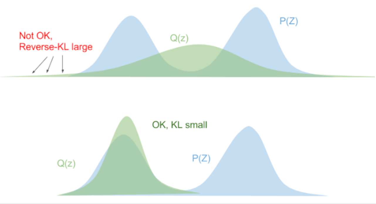
Here is a small point to note. Since the KL divergence is asymmetric, why do we minimize $D_{KL}(q_\phi\vert\vert p_\theta)$ rather than $D_{KL}(p_\theta\vert\vert q_\phi)$? (See this article for details.)
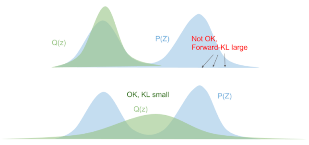
$D_{KL}(p_\theta\vert\vert q_\phi)$ is also called Forward KL, while $D_{KL}(q_\phi\vert\vert p_\theta)$ is called Reversed KL. Expanding Forward KL gives:
$$ D_{KL}(p_\theta\vert\vert q_\phi) = \sum_z p_\theta(z)\log\frac{p_\theta(z)}{q_\phi(z)} $$For any $p_\theta(z) \gt 0$, we have $\lim_{q_\phi(z) \to 0} \log \frac{p_\theta(z)}{q_\phi(z)} \to \infty$, which means that when $q_\phi$ cannot cover $p_\theta$, the value of Forward KL becomes very large. So the resulting $q_\phi$ will cover the whole of $q_\theta$, as shown below:
Expanding Reversed KL gives:
$$ D_{KL}(q_\phi\vert\vert q_\theta) = \sum_z q_\phi(z)\log \frac{q_\phi(z)}{p_\theta(z)} $$In the formula above, when $p_\theta(z)$ is 0, $q_\phi(z)$ must also be 0, otherwise the value of the KL divergence becomes abnormal. So the resulting $q_\phi$ is confined within the range of $p_\theta$, as shown below: