VQGAN is a generative model that performs well on a variety of image generation tasks (such as unconditional image generation, image completion, conditionally guided image generation and so on), the biggest highlight being image generation at the megapixel level.
The overall pipeline of the model is as follows:
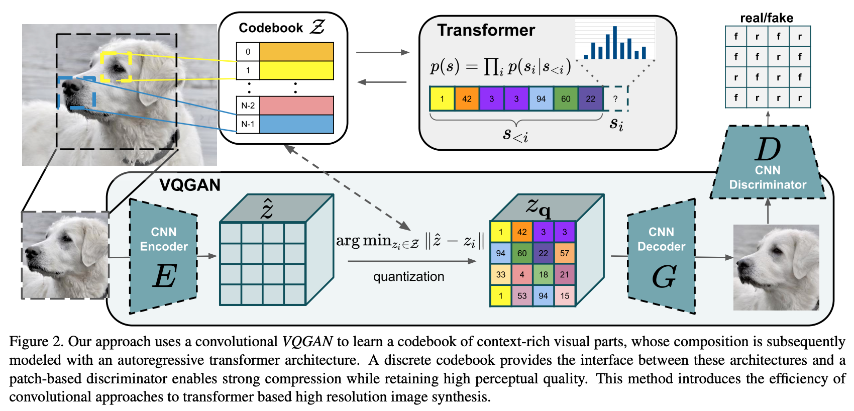
Overall it is similar to VQVAE, but the PixelCNN in VQVAE is replaced by a Transformer, and a PatchGAN discriminator is added during training to provide an adversarial loss.
Loss function
In VQVAE, the loss function can be expressed as follows:
$$ \begin{aligned} L_{VQ}(E,G,Z) &= L_{rec} + \vert\vert\text{sg}[E(x)] - z_q\vert\vert_2^2 + \vert\vert\text{sg}[z_q] - E(x)\vert\vert_2^2 \\ &= \vert\vert x - \hat{x}\vert\vert_2^2 + \vert\vert\text{sg}[E(x)] - z_q\vert\vert_2^2 + \vert\vert\text{sg}[z_q] - E(x)\vert\vert_2^2 \end{aligned} $$where $E,G,Z$ denote the encoder, decoder and codebook respectively. $\text{sg}$ is the stop gradient operation. $L_{rec}$ is the reconstruction loss.
In VQGAN, the authors replace $L_{rec}$ with a perceptual loss and also add the adversarial loss from GANs. In practice, to achieve better results on a particular task, the L2 loss may be used together with the perceptual loss, or the L2 loss may even be replaced by an L1 loss, which needs to be determined experimentally for each specific task.
Perceptual loss
In tasks such as image style transfer and super-resolution, traditional pixel-loss functions (such as L1, L2 or cross entropy) all pursue equality between the model output and the target at the pixel level, but a very small deviation in pixel values makes essentially no difference in actual appearance while the value of the pixel-loss becomes very large. The perceptual loss mainly focuses on features such as style, color and texture of the image, which better reflects the model’s optimization objective.
Computing this loss function requires an extra network to extract features; the concrete computation flow is roughly as follows:
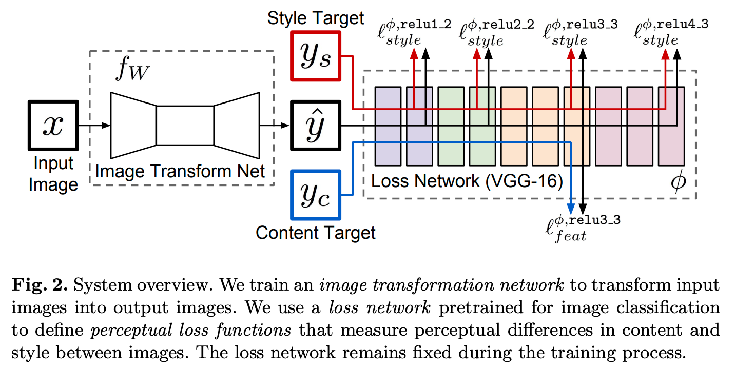
$f_W$ in the figure corresponds to the model we need to train. VGG-16 is a model pretrained on Imagenet, mainly used to extract features and not involved in weight updates. The perceptual loss is divided into two parts: content loss and style loss.
content loss is the L2 loss at the feature level. Computing it at the feature level rather than on the original image is meant to avoid the output becoming excessively similar to the target while still keeping the ability to guide the update of the content in the output. The mathematical expression is as follows:
$$ L^{\phi, j}_{feat}(\hat{y}, y) = \frac{1}{C_jH_jW_j}\vert\vert \phi_j(\hat{y}) - \phi_j(y)\vert\vert_2^2 $$where $\phi_j(\hat{y})$ and $\phi_j(y)$ denote the output features of the model output $\hat{y}$ and the target $y$ at the $j$-th layer of the VGG-16 network, with $\phi_j(\hat{y}), \phi_j(y)\in\mathbb{R}^{H_j\times W_j\times C_j}$. As can be seen from the figure above, the feature layer extracted in the paper is the output of relu3_3.
style loss is used to compute the differences between images in style, color, texture and so on. Suppose $\phi_j(x)\in\mathbb{R}^{H_j\times W_j\times C_j}$ denotes the output feature of input $x$ at the $j$-th layer of the model $\phi$. Here a Gram matrix $G_j^\phi(x)$ of size $C_j\times C_j$ is first defined:
$$ G_j^\phi(x)_{c,c^\prime} = \frac{1}{C_jH_jW_j}\sum^{H_j}_{h=1}\sum^{W_j}_{w=1}\phi_j(x)_{h,w,c}\phi_j(x)_{h,w,c^\prime} $$In actual computation we can reshape $\phi_j(x)$ to $\psi\in\mathbb{R}^{C_j\times H_jW_j}$, and then the Gram matrix computation simplifies as follows:
$$ G^\phi_j(x) = \frac{\psi\psi^T}{C_jH_jW_j} $$The style loss is defined as the Frobenius norm distance on the Gram matrix:
$$ L_{style}^{\phi,j}(\hat{y},y) = \vert\vert G_j^\phi(\hat{y}) - G_j^\phi(y)\vert\vert_F^2 $$The size of the output of the Gram matrix computation depends only on the number of channels of the input (the output size is $C_j\times C_j$), so as long as the number of channels is the same, the loss can be computed even if the sizes of the model output and the target differ.
In the feature extraction network, convolution layers at different depths extract different features (lower layers extract point and line features while higher layers extract abstract features), so in order to comprehensively evaluate the model’s style ability we need to extract the outputs of various network layers to compute the style loss. According to the figure above, the authors extract the output features of the four layers relu1_2, relu2_2, relu3_3 and relu4_3 to compute the style loss, and finally sum them as the value of the style loss.
As for the Frobenius norm, its computation formula is as follows ($A\in\mathbb{R}^{m\times n}$):
$$ \vert\vert A\vert\vert_F = \sqrt{\sum^m_{i=1}\sum^n_{j=1}\vert a_{ij}\vert^2} = \sqrt{\text{trace}(A^\star A)} = \sqrt{\sum_{i=1}^{\min(m,n)}\sigma_i^2} $$Three ways of computing the Frobenius norm are given above. Here $A^\star$ denotes the conjugate transpose of $A$ (the conjugate transpose swaps rows and columns and then conjugates each element; for a real matrix the conjugate transpose is just the transpose), and $\sigma_i$ are the singular values of $A$, using the trace function.
Adversarial loss
As for the adversarial loss part, the authors chose the Hinge loss suited to GANs. The ordinary Hinge loss is usually used in maximal margin classifiers such as support vector machines, improving model performance by widening as much as possible the score gap between positive and negative samples. Its mathematical expression is as follows:
$$ L = \max(0, 1-\hat{y}y) $$where $\hat{y}$ denotes the score the model outputs for a sample and $y$ denotes the ground truth label of the sample (1 or -1).
- When $\hat{y}$ and $y$ have the same sign, that is, the predicted class matches the true class: if $\vert\hat{y}\vert\le 1$, it means the margin is not large enough, so the loss is not 0 and updating continues until $\vert\hat{y}\vert\gt 1$, where the loss becomes 0
- When $\hat{y}$ and $y$ have opposite signs, that is, the predicted class differs from the true class, the loss is not 0
In Geometric GAN, the Hinge loss is introduced and transformed into the following form:
$$ \begin{aligned} L(G,D) &= L(G) + L(D) \\ &= -E(D(G(z))) + E(\max(0, 1-D(x))) + E(\max(0, 1+D(G(z)))) \end{aligned} $$The Hinge loss is mainly applied to the discriminator $D$. Only real samples with $D(x)\lt 1$ and generated samples with $D(G(z))\gt -1$ produce a loss, that is, only samples that are unreasonably classified contribute, which makes GAN training more stable.
In VQGAN, the adversarial loss is loosely expressed as follows:
$$ L_{GAN}(\{E,G,Z\}, D) = [\log(D(x)) + \log(1-D(\hat{x}))] $$Our goal is to obtain the optimal $E, G, Z$; the final summarized optimization objective is as follows:
$$ Q^\star = argmin_{E,G,Z}\max_D\mathbb{E}_{x\sim p(x)}[L_{VQ}(E,G,Z) + \lambda L_{GAN}(\{E,G,Z\}, D)] $$where $\lambda$ is an adaptive weight, expressed as follows:
$$ \lambda = \frac{\nabla_{G_L}[L_{rec}]}{\nabla_{G_L}[L_{GAN}]+\delta} $$$L_{rec}$ is the perceptual loss, $\nabla_{G_L}[\cdot]$ is a function denoting the gradient of the input of that function with respect to the last layer $L$ of the model decoder, and $\delta=10^{-6}$ is to prevent division by zero.
The newly added discriminator $D$ in VQGAN has the structure of a PatchGAN discriminator, which is a fully convolutional model structure. A usual GAN discriminator outputs only a single value, whereas a PatchGAN discriminator outputs an $n\times n$ matrix in which each value represents the score of the corresponding small region (patch) of the image for the input model. This design lets the model focus more on the details of the image and no longer evaluates the realism of an image with a single value.
Random image generation
The optimization objective above is already enough to train the various modules of the model, but in the random image generation task we need to sample $z_q$ and feed it to the decoder without an encoder. The VQVAE method predicts $z_q$ with PixelCNN. Considering that a Transformer has long-distance attention and that this sampling process can also be compared to the text sequence prediction problem, the authors use a Transformer-structure model to predict $z_q$ (specifically, the structure is GPT-2).
The sampling process is treated as autoregressive prediction, that is, the model is made to predict the distribution $p(s)=\prod_i p(s_i\vert s_{\lt i})$, and the corresponding loss function maximizes the log-likelihood:
$$ L_{Transformer} = \mathbb{E}_{x\sim p(x)}[-\log p(s)] $$The Transformer module needs to be trained after the other modules have been trained; the concrete training process is as follows:
- The input is passed through the encoder and the codebook to obtain $z_q\in \mathbb{R}^{h\times w\times n}$, which is unfolded into a 2D form $z_q^\prime\in \mathbb{R}^{hw\times n}$, that is, $hw$ codes of dimension $n$. The indices in the codebook corresponding to the combination of codes in $z_q^\prime$ at this point are defined as unmodified_indices
- Some of the codes in $z_q^\prime$ are replaced with randomly generated codes (still of dimension $n$), and the indices corresponding to the modified combination of codes are defined as modified_indices. Replacing with random codes amounts to adding noise to the features, which improves the generalization of the Transformer
- The modified_indices are fed into the Transformer model, and the model is trained with a cross-entropy loss to reconstruct the unmodified_indices
With the help of the Transformer, VQGAN achieves image generation at the megapixel level.
Reference
Taming Transformers for High-Resolution Image Synthesis
Perceptual Losses for Real-Time Style Transfer and Super-Resolution
Image-to-Image Translation with Conditional Adversarial Networks
Megapixel image generation combining discretized coding and Transformers