This is an image generation model of the diffusion model type. To put it simply, by continuously adding Gaussian noise to the original image $\mathbf{x}_0$ ($T$ rounds in total), $\mathbf{x}_0$ can finally be turned into pure Gaussian noise $\mathbf{x}_T$, and the model is responsible for restoring $\mathbf{x}_T$ to $\mathbf{x}_0$. This is illustrated below:

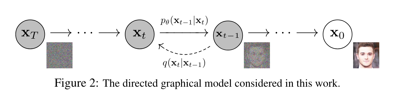
Here the process from $\mathbf{x}_0$ to $\mathbf{x}_T$ is called the forward process, and the process from $\mathbf{x}_T$ to $\mathbf{x}_0$ is the reverse or inference process.

Most of this post is based on What are Diffusion Models.

Forward process

Given the input image $\mathbf{x}_0 \sim q(\mathbf{x})$, $T$ rounds of Gaussian noise are added to obtain $\mathbf{x}_1$, $\mathbf{x}_2$, $\dots$, $\mathbf{x}_T$. In this process $\mathbf{x}_t$ depends only on $\mathbf{x}_{t-1}$, so it can be regarded as a Markov process. We have:

$$ \begin{aligned} q(\mathbf{x}_t \vert \mathbf{x}_{t-1}) &= \mathcal{N}(\mathbf{x}_t; \sqrt{1 - \beta_t} \mathbf{x}_{t-1}, \beta_t\mathbf{I}) \\ q(\mathbf{x}_{1:T} \vert \mathbf{x}_0) &= \prod^T_{t=1} q(\mathbf{x}_t \vert \mathbf{x}_{t-1}) \end{aligned} $$

where $\{\beta_t\in (0, 1)\}^T_{t=1}$ are given hyperparameters denoting the variances of a series of Gaussian distributions. In practice $\beta_t$ increases as $t$ grows.

Let $\alpha_t = 1 - \beta_t$ and $\overline{\alpha}_t = \Pi_{i=1}^t\alpha_i$. Using the reparameterization trick we have:

$$ \begin{aligned} \mathbf{x}_t &= \sqrt{\alpha_t}\mathbf{x}_{t-1} + \sqrt{1 - \alpha_t}\boldsymbol{\epsilon}_{t-1} \\ &= \sqrt{\alpha_t \alpha_{t-1}} \mathbf{x}_{t-2} + \sqrt{1 - \alpha_t \alpha_{t-1}} \bar{\boldsymbol{\epsilon}}_{t-2} & \\ &= \dots \\ &= \sqrt{\bar{\alpha}_t}\mathbf{x}_0 + \sqrt{1 - \bar{\alpha}_t}\boldsymbol{\epsilon} \\ q(\mathbf{x}_t \vert \mathbf{x}_0) &= \mathcal{N}(\mathbf{x}_t; \sqrt{\bar{\alpha}_t} \mathbf{x}_0, (1 - \bar{\alpha}_t)\mathbf{I}) \end{aligned} $$

where $\boldsymbol{\epsilon}_{t-1}, \boldsymbol{\epsilon}_{t-2}, \dots \sim \mathcal{N}(\mathbf{0}, \mathbf{I})$ and $\bar\epsilon_{t-2}$ denotes the combination of two Gaussian distributions, that is, combining them through the additivity of independent Gaussian distributions:

$$ \mathcal{N}(\mathbf{0}, \sigma_2^2\mathbf{I}) + \mathcal{N}(\mathbf{0}, \sigma_2^2\mathbf{I}) \sim \mathcal{N}(\mathbf{0}, (\sigma^2_1+\sigma^2_2)\mathbf{I}) $$

In summary we obtain:

$$ \begin{aligned} \mathbf{x}_t = \sqrt{\overline{\alpha}_t}\mathbf{x}_0 + \sqrt{1-\overline{\alpha}_t}\boldsymbol\epsilon \end{aligned} \tag{1} $$

that is, $\mathbf{x}_t$ at any time step can be expressed in terms of $\mathbf{x}_0$ and $\beta$. At the same time, from (1) we can see that as $t$ grows, $\beta_t$ also grows and $\overline\alpha_t$ gets closer to 0, so $\mathbf{x}_t$ gets closer to the standard Gaussian distribution $\mathcal{N}(\mathbf{0}, \mathbf{I})$.

Reverse process

If we could obtain the reversed distribution $q(\mathbf{x}_{t-1} \vert \mathbf{x}_t)$, we could restore $\mathbf{x}_0$ from the completely standard Gaussian distribution $\mathbf{x}_t\sim\mathcal{N}(\mathbf{0}, \mathbf{I})$. Note that when $\beta_t$ is small enough, $q(\mathbf{x}_{t-1}\vert\mathbf{x}_t)$ is still a Gaussian distribution, but usually we cannot easily infer $q(\mathbf{x}_{t-1}\vert\mathbf{x}_t)$, so we use a deep learning model (parameterized by $\theta$, with the current mainstream structure being Unet + Attention) to predict a distribution $p_\theta$ that approximates $q(\mathbf{x}_{t-1}\vert\mathbf{x}_t)$.

$$ \begin{aligned} p_\theta(\mathbf{x}_{0:T}) &= p(\mathbf{x}_T) \prod^T_{t=1} p_\theta(\mathbf{x}_{t-1} \vert \mathbf{x}_t) \\ p_\theta(\mathbf{x}_{t-1} \vert \mathbf{x}_t) &= \mathcal{N}(\mathbf{x}_{t-1}; \boldsymbol{\mu}_\theta(\mathbf{x}_t, t), \boldsymbol{\Sigma}_\theta(\mathbf{x}_t, t)) \end{aligned} $$

From the formulas above we can see that, to obtain the distribution $p_\theta$, $\boldsymbol{\mu}_\theta(\mathbf{x}_t, t)$ and $\boldsymbol{\Sigma}_\theta(\mathbf{x}_t, t)$ are needed.

For the reversed distribution $q(\mathbf{x}_{t-1}\vert\mathbf{x}_t)$, adding $\mathbf{x}_0$ as a known condition gives:

$$ q(\mathbf{x}_{t-1} \vert \mathbf{x}_t, \mathbf{x}_0) = \mathcal{N}(\mathbf{x}_{t-1}; {\tilde{\boldsymbol{\mu}}}(\mathbf{x}_t, \mathbf{x}_0), {\tilde{\beta}_t} \mathbf{I}) $$

The variance is written as $\tilde{\beta_t}$ because the DDPM paper simplifies things by setting $\boldsymbol{\Sigma}_\theta(\mathbf{x}_t, t)$ directly to $\tilde{\beta_t}$.

By Bayes’ formula we obtain:

$$ q(\mathbf{x}_{t-1}\vert\mathbf{x}_t,\mathbf{x}_0) = \frac{q(\mathbf{x}_t\vert\mathbf{x}_{t-1},\mathbf{x}_0)q(\mathbf{x}_{t-1}\vert\mathbf{x}_0)}{q(\mathbf{x}_t\vert\mathbf{x}_0)} $$

that is, the reverse process is entirely converted into the forward process. Substituting the density function of the Gaussian distribution gives:

$$ \begin{aligned} & q(\mathbf{x}_{t-1} \vert \mathbf{x}_t, \mathbf{x}_0) \\ = & \frac{q(\mathbf{x}_t\vert\mathbf{x}_{t-1},\mathbf{x}_0)q(\mathbf{x}_{t-1}\vert\mathbf{x}_0)}{q(\mathbf{x}_t\vert\mathbf{x}_0)} \\ \propto & \exp\Big( -\frac{1}{2} \big( (\frac{\alpha_t}{\beta_t} + \frac{1}{1 - \bar{\alpha}_{t-1}}) \mathbf{x}_{t-1}^2 - (\frac{2\sqrt{\alpha_t}}{\beta_t} \mathbf{x}_t + \frac{2\sqrt{\bar{\alpha}_{t-1}}}{1 - \bar{\alpha}_{t-1}} \mathbf{x}_0) \mathbf{x}_{t-1} + C(\mathbf{x}_t, \mathbf{x}_0) \big) \Big) \end{aligned} $$

The density function of an ordinary Gaussian distribution $\mathcal{N}(\mu, \sigma^2)$ is as follows:

$$ \begin{aligned} f(x) &= \frac{1}{\sqrt{2\pi}\sigma}\exp(-\frac{(x-\mu)^2}{2\sigma^2}) \\ &=\frac{1}{\sqrt{2\pi}\sigma}\exp(-\frac{1}{2}(\frac{1}{\sigma^2}x^2-\frac{2\mu}{\sigma^2}x+\frac{\mu^2}{\sigma^2})) \end{aligned} $$

Comparing with the formula above, we have:

$$ \begin{aligned} \frac{1}{\sigma^2} &= \frac{1}{\tilde{\beta}_t} = \frac{\alpha_t}{\beta_t}+\frac{1}{1-\bar\alpha_{t-1}} \\ &\Rightarrow \tilde{\beta}_t = \frac{1-\bar\alpha_{t-1}}{1-\bar\alpha_t}\cdot\beta_t \\ \frac{2\mu}{\sigma^2} &= \frac{2\sqrt{\alpha_t}}{\beta_t} \mathbf{x}_t + \frac{2\sqrt{\bar{\alpha}_{t-1}}}{1 - \bar{\alpha}_{t-1}} \mathbf{x}_0 \\ &\Rightarrow \tilde\mu_t(\mathbf{x}_t, \mathbf{x}_0) = \frac{\sqrt{\alpha_t}(1-\bar\alpha_{t-1})}{1-\bar\alpha_t}\mathbf{x}_t+\frac{\sqrt{\bar\alpha_{t-1}}\beta_t}{1-\bar\alpha_t}\mathbf{x}_0 \end{aligned} $$

So the variance $\tilde{\beta}_t$ is a constant, while the mean $\tilde\mu_t$ depends on $\mathbf{x}_t$ and $\mathbf{x}_0$. From (1) we obtain $\mathbf{x}_0 = \frac{1}{\sqrt{\bar{\alpha}_t}}(\mathbf{x}_t - \sqrt{1 - \bar{\alpha}_t}\boldsymbol{\epsilon}_t)$, and substituting into the formula above gives:

$$ \begin{aligned} \tilde{\boldsymbol{\mu}}_t =\frac{1}{\sqrt{\alpha_t}} \Big( \mathbf{x}_t - \frac{1 - \alpha_t}{\sqrt{1 - \bar{\alpha}_t}} \boldsymbol{\epsilon}_t \Big) \end{aligned} \tag{2} $$

where the Gaussian distribution $\boldsymbol{\epsilon}_t$ in the model is the predicted noise distribution, $\boldsymbol{\epsilon}_\theta(\mathbf{x}_t, t)$, so we have:

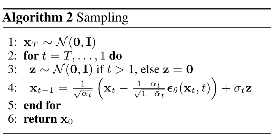
$$ \begin{aligned} \boldsymbol{\mu}_\theta(\mathbf{x}_t, t) =\frac{1}{\sqrt{\alpha_t}} \Big( \mathbf{x}_t - \frac{1 - \alpha_t}{\sqrt{1 - \bar{\alpha}_t}} \boldsymbol{\epsilon}_\theta(\mathbf{x}_t, t) \Big) \end{aligned} \tag{3} $$

Putting the reverse process above together, we obtain the model inference steps as follows:

• The model predicts the Gaussian noise $\boldsymbol{\epsilon}_\theta(\mathbf{x}_t, t)$ from $\mathbf{x}_t$ and $t$, and then $\boldsymbol{\mu}_\theta(\mathbf{x}_t, t)$ is obtained from (3)
• Compute the variance $\Sigma_\theta(\mathbf{x}_t, t)$. DDPM replaces $\Sigma_\theta(\mathbf{x}_t, t)$ with $\tilde\beta_t$ and considers $\beta_t$ and $\tilde\beta_t$ to be approximately equal
• $\mathbf{x}_{t-1}$ is obtained from $p_\theta(\mathbf{x}_{t-1} \vert \mathbf{x}_t) = \mathcal{N}(\mathbf{x}_{t-1}; \boldsymbol{\mu}_\theta(\mathbf{x}_t, t), \boldsymbol{\Sigma}_\theta(\mathbf{x}_t, t))$ using the reparameterization method

The DDPM inference procedure is as follows:

Training process

As mentioned above, we use a model to predict a distribution $p_\theta(\mathbf{x}_{t-1}\vert\mathbf{x}_t)$ that approximates the reversed distribution $q(\mathbf{x}_{t-1}\vert\mathbf{x}_t)$. There are generally two ways to approach this problem: one is to optimize the maximum likelihood of the negative log, $-\log p_\theta(\mathbf{x}_0)$; the other is to optimize the cross entropy between the predicted distribution and the true distribution, $\mathbb{E}_{q(\mathbf{x}_0)}[-\log p_\theta(\mathbf{x}_0)]$. Both are rather difficult to optimize directly, so we consider optimizing their variational lower bound (VLB) instead.

Since the KL divergence is non-negative, we have:

$$ -\log p_\theta(\mathbf{x}_0) \leq -\log p_\theta(\mathbf{x}_0) + D_{KL}(q(\mathbf{x}_{1:T}\vert\mathbf{x}_0)\vert\vert p_\theta(\mathbf{x}_{1:T}\vert\mathbf{x}_0)) $$

Expanding and simplifying the KL divergence, and taking the expectation $\mathbb{E}_{q(\mathbf{x}_0)}$ on both sides, gives:

$$ \begin{aligned} \mathcal{L}_{VLB} &= \mathbb{E}_{q(\mathbf{x}_0)}\Big( -\log p_\theta(\mathbf{x}_0) + \mathbb{E}_{q(\mathbf{x}_{1:T}\vert\mathbf{x}_0)}\Big[\log\frac{q(\mathbf{x}_{1:T}\vert\mathbf{x}_0)}{p_\theta(\mathbf{x}_{0:T})} + \log p_\theta (\mathbf{x}_0)\Big]\Big)\\ &= \mathbb{E}_{q(\mathbf{x}_0)}\Big( \mathbb{E}_{q(\mathbf{x}_{1:T}\vert\mathbf{x}_0)}\Big[\log\frac{q(\mathbf{x}_{1:T}\vert\mathbf{x}_0)}{p_\theta(\mathbf{x}_{0:T})}\Big]\Big) \\ &= \mathbb{E}_{q(\mathbf{x}_{0:T})}\Big[\log\frac{q(\mathbf{x}_{1:T}\vert\mathbf{x}_0)}{p_\theta(\mathbf{x}_{0:T})}\Big] \\ &\geq \mathbb{E}_{q(\mathbf{x}_0)}[-\log p_\theta(\mathbf{x}_0)] \end{aligned} $$

The second equality above uses Fubini’s theorem, and Jensen’s inequality gives the same result:

$$ \begin{aligned} & \mathbb{E}_{q(\mathbf{x}_0)}[-\log p_\theta(\mathbf{x}_0)] \\ =& -\mathbb{E}_{q(\mathbf{x}_0)}\Big[\log\Big(p_\theta(\mathbf{x}_0)\cdot\int p_\theta(\mathbf{x}_{1:T})d\mathbf{x}_{1:T}\Big)\Big] \\ =& -\mathbb{E}_{q(\mathbf{x}_0)}\Big[\log\Big(\int p_\theta(\mathbf{x}_{0:T})d\mathbf{x}_{1:T}\Big)\Big] \\ =& -\mathbb{E}_{q(\mathbf{x}_0)}\Big[\log\Big(\int q(\mathbf{x}_{1:T}\vert\mathbf{x}_0)\frac{p_\theta(\mathbf{x}_{0:T})}{q(\mathbf{x}_{1:T}\vert\mathbf{x}_0)}d\mathbf{x}_{1:T}\Big)\Big] \\ =& -\mathbb{E}_{q(\mathbf{x}_{0:T})}\Big[\log\Big(\mathbb{E}_{q(\mathbf{x}_{1:T}\vert\mathbf{x}_0)}\frac{p_\theta(\mathbf{x}_{0:T})}{q(\mathbf{x}_{1:T}\vert\mathbf{x}_0)}\Big)\Big] \\ \leq & -\mathbb{E}_{q(\mathbf{x}_{0:T})}\Big[\log\frac{p_\theta(\mathbf{x}_{0:T})}{q(\mathbf{x}_{1:T}\vert\mathbf{x}_0)}\Big] \\ =& \mathbb{E}_{q(\mathbf{x}_{0:T})}\Big[\log\frac{q(\mathbf{x}_{1:T}\vert\mathbf{x}_0)}{p_\theta(\mathbf{x}_{0:T})}\Big] = \mathcal{L}_{VLB} \end{aligned} $$

Note that $\log$ is a concave function, so $-\log$ is convex.

Thus we finally obtain:

$$ \mathcal{L}_{VLB} = \mathbb{E}_{q(\mathbf{x}_{0:T})}\Big[\log\frac{q(\mathbf{x}_{1:T}\vert\mathbf{x}_0)}{p_\theta(\mathbf{x}_{0:T})}\Big] \geq \mathbb{E}_{q(\mathbf{x}_0)}[-\log p_\theta(\mathbf{x}_0)] $$

So minimizing $\mathbf{L}_{VLB}$ minimizes the target loss function $\mathbb{E}_{q(\mathbf{x}_0)}[-\log p_\theta(\mathbf{x}_0)]$.

Deriving $\mathbf{L}_{VLB}$ gives:

$$ \begin{aligned} \mathcal{L}_{VLB} &= \mathbb{E}_{q(\mathbf{x}_{0:T})} \Big[ \log\frac{q(\mathbf{x}_{1:T}\vert\mathbf{x}_0)}{p_\theta(\mathbf{x}_{0:T})} \Big] \\ &= \mathbb{E}_q \Big[ \log\frac{\prod_{t=1}^T q(\mathbf{x}_t\vert\mathbf{x}_{t-1})}{ p_\theta(\mathbf{x}_T) \prod_{t=1}^T p_\theta(\mathbf{x}_{t-1} \vert\mathbf{x}_t) } \Big] \\ &= \mathbb{E}_q \Big[ -\log p_\theta(\mathbf{x}_T) + \sum_{t=1}^T \log \frac{q(\mathbf{x}_t\vert\mathbf{x}_{t-1})}{p_\theta(\mathbf{x}_{t-1} \vert\mathbf{x}_t)} \Big] \\ &= \mathbb{E}_q \Big[ -\log p_\theta(\mathbf{x}_T) + \sum_{t=2}^T \log \frac{q(\mathbf{x}_t\vert\mathbf{x}_{t-1})}{p_\theta(\mathbf{x}_{t-1} \vert\mathbf{x}_t)} + \log\frac{q(\mathbf{x}_1 \vert \mathbf{x}_0)}{p_\theta(\mathbf{x}_0 \vert \mathbf{x}_1)} \Big] \\ &= \mathbb{E}_q \Big[ -\log p_\theta(\mathbf{x}_T) + \sum_{t=2}^T \log \Big( \frac{q(\mathbf{x}_{t-1} \vert \mathbf{x}_t, \mathbf{x}_0)}{p_\theta(\mathbf{x}_{t-1} \vert\mathbf{x}_t)}\cdot \frac{q(\mathbf{x}_t \vert \mathbf{x}_0)}{q(\mathbf{x}_{t-1}\vert\mathbf{x}_0)} \Big) + \log \frac{q(\mathbf{x}_1 \vert \mathbf{x}_0)}{p_\theta(\mathbf{x}_0 \vert \mathbf{x}_1)} \Big] \\ &= \mathbb{E}_q \Big[ -\log p_\theta(\mathbf{x}_T) + \sum_{t=2}^T \log \frac{q(\mathbf{x}_{t-1} \vert \mathbf{x}_t, \mathbf{x}_0)}{p_\theta(\mathbf{x}_{t-1} \vert\mathbf{x}_t)} + \sum_{t=2}^T \log \frac{q(\mathbf{x}_t \vert \mathbf{x}_0)}{q(\mathbf{x}_{t-1} \vert \mathbf{x}_0)} + \log\frac{q(\mathbf{x}_1 \vert \mathbf{x}_0)}{p_\theta(\mathbf{x}_0 \vert \mathbf{x}_1)} \Big] \\ &= \mathbb{E}_q \Big[ -\log p_\theta(\mathbf{x}_T) + \sum_{t=2}^T \log \frac{q(\mathbf{x}_{t-1} \vert \mathbf{x}_t, \mathbf{x}_0)}{p_\theta(\mathbf{x}_{t-1} \vert\mathbf{x}_t)} + \log\frac{q(\mathbf{x}_T \vert \mathbf{x}_0)}{q(\mathbf{x}_1 \vert \mathbf{x}_0)} + \log \frac{q(\mathbf{x}_1 \vert \mathbf{x}_0)}{p_\theta(\mathbf{x}_0 \vert \mathbf{x}_1)} \Big]\\ &= \mathbb{E}_q \Big[ \log\frac{q(\mathbf{x}_T \vert \mathbf{x}_0)}{p_\theta(\mathbf{x}_T)} + \sum_{t=2}^T \log \frac{q(\mathbf{x}_{t-1} \vert \mathbf{x}_t, \mathbf{x}_0)}{p_\theta(\mathbf{x}_{t-1} \vert\mathbf{x}_t)} - \log p_\theta(\mathbf{x}_0 \vert \mathbf{x}_1) \Big] \\ &= \mathbb{E}_q [\underbrace{D_\text{KL}(q(\mathbf{x}_T \vert \mathbf{x}_0) \parallel p_\theta(\mathbf{x}_T))}_{L_T} + \sum_{t=2}^T \underbrace{D_\text{KL}(q(\mathbf{x}_{t-1} \vert \mathbf{x}_t, \mathbf{x}_0) \parallel p_\theta(\mathbf{x}_{t-1} \vert\mathbf{x}_t))}_{L_{t-1}} \underbrace{- \log p_\theta(\mathbf{x}_0 \vert \mathbf{x}_1)}_{L_0} ] \end{aligned} $$

that is, $\mathcal{L}_{VLB}$ is turned into a sum of several entropies or KL divergences. Finally it is expressed as:

$$ \begin{aligned} \mathcal{L}_{VLB} &= L_T + L_{T-1} + \dots + L_0 \\ \text{where } L_T &= D_\text{KL}(q(\mathbf{x}_T \vert \mathbf{x}_0) \parallel p_\theta(\mathbf{x}_T)) \\ L_t &= D_\text{KL}(q(\mathbf{x}_t \vert \mathbf{x}_{t+1}, \mathbf{x}_0) \parallel p_\theta(\mathbf{x}_t \vert\mathbf{x}_{t+1})) \text{ for }1 \leq t \leq T-1 \\ L_0 &= - \log p_\theta(\mathbf{x}_0 \vert \mathbf{x}_1) \end{aligned} $$

The forward process $q$ has no learnable parameters, and $\mathbf{x}_T$ is pure Gaussian noise, so $L_T$ can be treated as a constant. $L_t$ can be regarded as closing the distance between two Gaussian distributions; from solving the KL divergence of multivariate Gaussian distributions we have:

$$ \mathcal{L}_{VLB} = \mathbb{E}_q\Big[\frac{1}{2{\vert\vert\Sigma_\theta(\mathbf{x}_t, t)\vert\vert}^2_2}{\vert\vert\tilde\mu_t(\mathbf{x}_t, \mathbf{x}_0)-\mu_\theta(\mathbf{x}_t, t)\vert\vert}^2\Big] + C $$

where $C$ is unrelated to the model parameters. Substituting $(1), (2), (3)$ into the formula above gives:

$$ \begin{aligned} L_t &= \mathbb{E}_{\mathbf{x}_0, \boldsymbol{\epsilon}} \Big[\frac{1}{2 \| \boldsymbol{\Sigma}_\theta(\mathbf{x}_t, t) \|^2_2} \| \tilde{\boldsymbol{\mu}}_t(\mathbf{x}_t, \mathbf{x}_0) - \boldsymbol{\mu}_\theta(\mathbf{x}_t, t) \|^2 \Big] \\ &= \mathbb{E}_{\mathbf{x}_0, \boldsymbol{\epsilon}} \Big[\frac{1}{2 \|\boldsymbol{\Sigma}_\theta \|^2_2} \| \frac{1}{\sqrt{\alpha_t} \Big( \mathbf{x}_t - \frac{1 - \alpha_t}{\sqrt{1 - \bar{\alpha}_t}} \boldsymbol{\epsilon}_t \Big)} - \frac{1}{\sqrt{\alpha_t}} \Big( \mathbf{x}_t - \frac{1 - \alpha_t}{\sqrt{1 - \bar{\alpha}_t} \boldsymbol{\boldsymbol{\epsilon}}_\theta(\mathbf{x}_t, t) \Big)} \|^2 \Big] \\ &= \mathbb{E}_{\mathbf{x}_0, \boldsymbol{\epsilon}} \Big[\frac{ (1 - \alpha_t)^2 }{2 \alpha_t (1 - \bar{\alpha}_t) \| \boldsymbol{\Sigma}_\theta \|^2_2} \|\boldsymbol{\epsilon}_t - \boldsymbol{\epsilon}_\theta(\mathbf{x}_t, t)\|^2 \Big] \\ &= \mathbb{E}_{\mathbf{x}_0, \boldsymbol{\epsilon}} \Big[\frac{ (1 - \alpha_t)^2 }{2 \alpha_t (1 - \bar{\alpha}_t) \| \boldsymbol{\Sigma}_\theta \|^2_2} \|\boldsymbol{\epsilon}_t - \boldsymbol{\epsilon}_\theta(\sqrt{\bar{\alpha}_t}\mathbf{x}_0 + \sqrt{1 - \bar{\alpha}_t}\boldsymbol{\epsilon}_t, t)\|^2 \Big] \end{aligned} $$

From the formula above we can see that the focus of model training is optimizing the MAE between the two Gaussian noises $\boldsymbol\epsilon$ and $\boldsymbol\epsilon_\theta$.

For $L_0$, DDPM designs a discretized piecewise integral accumulation for $p_\theta(\mathbf{x}_0\vert\mathbf{x}_1)$, and also simplifies $\mathcal{L}_{VLB}$ (ignoring the coefficients), giving:

$$ \begin{aligned} L_t^\text{simple} &= \mathbb{E}_{t \sim [1, T], \mathbf{x}_0, \boldsymbol{\epsilon}_t} \Big[\|\boldsymbol{\epsilon}_t - \boldsymbol{\epsilon}_\theta(\mathbf{x}_t, t)\|^2 \Big] \\ &= \mathbb{E}_{t \sim [1, T], \mathbf{x}_0, \boldsymbol{\epsilon}_t} \Big[\|\boldsymbol{\epsilon}_t - \boldsymbol{\epsilon}_\theta(\sqrt{\bar{\alpha}_t}\mathbf{x}_0 + \sqrt{1 - \bar{\alpha}_t}\boldsymbol{\epsilon}_t, t)\|^2 \Big] \\ \Rightarrow & L_{simple} = L^{simple}_t + C \end{aligned} $$

As mentioned earlier, DDPM does not compute $\Sigma_\theta(\mathbf{x}_t, t)$ but uses a non-trainable $\beta_t$ or $\tilde\beta_t$. So the training procedure of DDPM is roughly as follows:

• Obtain $\mathbf{x}_0$, and randomly sample a $t$ from $1\dots T$
• Randomly sample a noise $\epsilon_t \sim \mathcal{N}(\mathbf{0}, \mathbf{I})$ from the standard Gaussian distribution
• Minimize $\|\boldsymbol{\epsilon}_t - \boldsymbol{\epsilon}_\theta(\sqrt{\bar{\alpha}_t}\mathbf{x}_0 + \sqrt{1 - \bar{\alpha}_t}\boldsymbol{\epsilon}_t, t) \|$

The DDPM training flow chart is as follows:

Appendix

A. Reparameterization

Usually the process of randomly sampling a sample from some distribution cannot be backpropagated through. Reparameterization uses an independent random variable to direct the randomness out.

Suppose $\mathbf{z}$ follows a Gaussian distribution with expectation $\mu_\theta$ and variance $\sigma_\theta^2$. Reparameterized sampling can be written in the following form:

$$ \mathbf{z} = \mu_\theta + \sigma_\theta \odot \epsilon, \quad \epsilon\sim\mathcal{N}(\mathbf{0}, \mathbf{I}) $$

where $\odot$ denotes element-wise multiplication. The formula above moves the randomness of $\mathbf{z}$ onto $\epsilon$ while still satisfying $\mathbf{z}\sim \mathcal{N}(\mathbf{z}; \mu_\theta, \sigma^2_\theta\mathbf{I})$, and this process is differentiable.

B. Jensen’s inequality

Let $x$ be a random variable and $\phi$ be a convex function; then the following holds:

$$ \phi(E(x)) \leq E(\phi(x)) $$

If $x$ is a discrete random variable, this can be written as: $\phi(\frac{1}{n}\sum x)\leq\frac{1}{n}\sum\phi(x)$

C. KL divergence

The KL divergence of the distributions $p(x)$ and $q(x)$ is denoted $D_{KL}(p\|q)$, and:

$$ D_{KL}(p\|q) = E_{p(x)}[\log\frac{p(x)}{q(x)}] $$

Jensen’s inequality can be used to show that the KL divergence is always greater than 0:

$$ \begin{aligned} D_{KL}(p\|q) &= E_{p(x)}[\log\frac{p(x)}{q(x)}] \\ &= E_{p(x)}[-\log\frac{q(x)}{p(x)}] \\ &\ge-\log\Big( E_{p(x)}[\frac{q(x)}{p(x)}] \Big) \\ &=-\log\Big(\int p(x)\frac{q(x)}{p(x)} dx\Big) \\ &=-\log\Big(\int q(x)dx\Big) \\ &=-\log(1) = 0 \end{aligned} $$

Reference

Denoising Diffusion Probabilistic Models

What are Diffusion Models

Understanding Diffusion Model from the ground up

Explaining Diffusion Model DDPM in one article

DDPM of diffusion models