Previous diffusion models (DM) generally operate over the full image, which makes the GPU memory required to run a DM model very large. The latent diffusion model (LDM), by contrast, maps the input to a latent space through a pretrained autoencoder encoder, performs the DM operations in that latent space, and finally maps the output back to the original image space through the autoencoder decoder. The authors also introduce the conditioning information into the DM through cross attention, thereby achieving controllable image generation.
Autoencoder
An autoencoder is a kind of neural network that learns in an unsupervised manner. It is trained by comparing the generated image with the original image, that is, it focuses on the model’s reconstruction ability; an AE model has no generative ability either. This network consists of two parts:
- Encoder: converts the original high-dimensional input data into a latent low-dimensional code. The input size is larger than the output size.
- Decoder: restores the latent low-dimensional code obtained by the encoder into the original input data.
In LDM, the authors use two optional regularization methods, $\text{KL-reg}$ and $\text{VQ-reg}$, to avoid the large variance that the latent space is very likely to exhibit. The loss functions used are the perceptual loss and a Discriminator loss that involves adversarial training.
- KL-reg: the autoencoder model under this penalty is called AutoencoderKL, which can be regarded as a standard VAE (with a KL loss). This model adds a small KL penalty to the learned latent variable so that it approaches a standard normal distribution.
- VQ-reg: this autoencoder model can be regarded as VQ-GAN, but the vector quantized layer is placed in the decoder.
Loss function
The perceptual loss in LDM uses the learnable Learned Perceptual Image Patch Similarity (LPIPS) to measure the difference between two images. The Discriminator loss borrows the training process of the taming transformer.
LPIPS
When computing image similarity, traditional methods such as L2, SSIM and PSNR differ considerably from human judgment, especially when images are smooth, where traditional methods are very likely to fail. The authors use deep learning network features to measure image similarity and verified the effectiveness of this design through a large number of experiments. Here the authors introduce two new evaluation metrics:
- 2AFC (two alternative forced choice): the experimenter is given one original image and two modified images, and must judge which one is closer to the original. A problem with this metric is that the experimenter may consciously choose which aspects of similarity to focus on.
- JND (just noticeable difference): the experimenter is shown two images in succession, each for 1 second with a 250-millisecond gap, and then asked to judge whether the two images are the same. Only asking the experimenter whether the two images are similar avoids, to some extent, the subjectivity of the experimenter’s choice when both images are partly similar.
The structure of LPIPS is shown below:
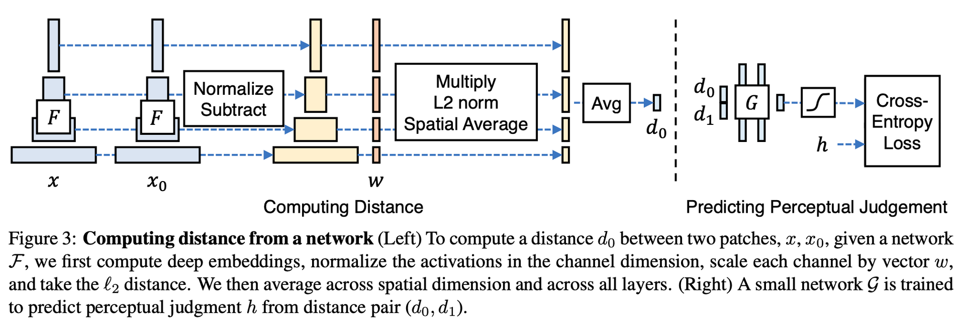
- The two patches $\mathbf{x}$ and $\mathbf{x}_0$ are fed separately into a feature extraction model $\mathcal{F}$, which can be a network such as VGG or AlexNet (VGG-16 in LDM)
- The outputs of different layers (more precisely, different stages) of $\mathcal{F}$ are extracted and normalized along the channel dimension to obtain $\hat{y}^l, \hat{y}^l \in \mathbb{R}^{H_l\times W_l\times C_l}$, where $l$ indicates that the output of the $l$-th layer is extracted
- $w^l\in\mathbb{R}^{C_l}$ is used to scale $\hat{y}^l$ and $\hat{y}^l$ per channel, after which their L2 distance is computed. Finally the average gives the result
The formula is described as follows:
$$ d(x,x_0)=\sum_l\frac{1}{H_lW_l}\sum_{h,w}\vert\vert w_l\odot(\hat{y}^l_{hw} - \hat{y}^l_{0hw})\vert\vert_2^2 $$When $w_l=1$ for $\forall l$, the formula above can be seen as the cosine distance.
During training, as shown in the figure above, the two distances are mainly used as the input of a small network $\mathcal{G}$ to compute a score $\hat{h}\in(0,1)$, and then the model is trained with a cross-entropy loss; $h$ in the figure is the new metric introduced by the authors, which here is 2AFC.
In the LPIPS paper, the authors give three ways of training the model:
- lin: fix the pretrained weights of $\mathcal{F}$ and train only the weights $w$
- tune: load the pretrained weights of $\mathcal{F}$ and train them together with $w$
- scratch: initialize the model weights with a random Gaussian distribution and train from scratch
Discriminator loss
A PatchGAN discriminator is used to obtain a patch-level realism evaluation of the image, which is optimized with an adversarial loss function. Referring to VQ-GAN, its loss function can be roughly expressed as follows:
$$ L_D = [\log(D(x)) + \log(1-D(\hat{x}))] $$where $D$ is the discriminator, $x$ is a real sample and $\hat{x}$ is a generated sample. For the details of this part, refer to VQ-GAN.
Conditoinal Denoiser
The DM part is similar to DDPM, in that a UNet also predicts the noise. Both the Latent Diffusion Model and Stable Diffusion adopt a time-conditional UNet structure to predict the noise at each step, but the official files do not provide a detailed UNet structure figure. Referring to another paper, the rough structure of the time-conditional UNet is as follows:
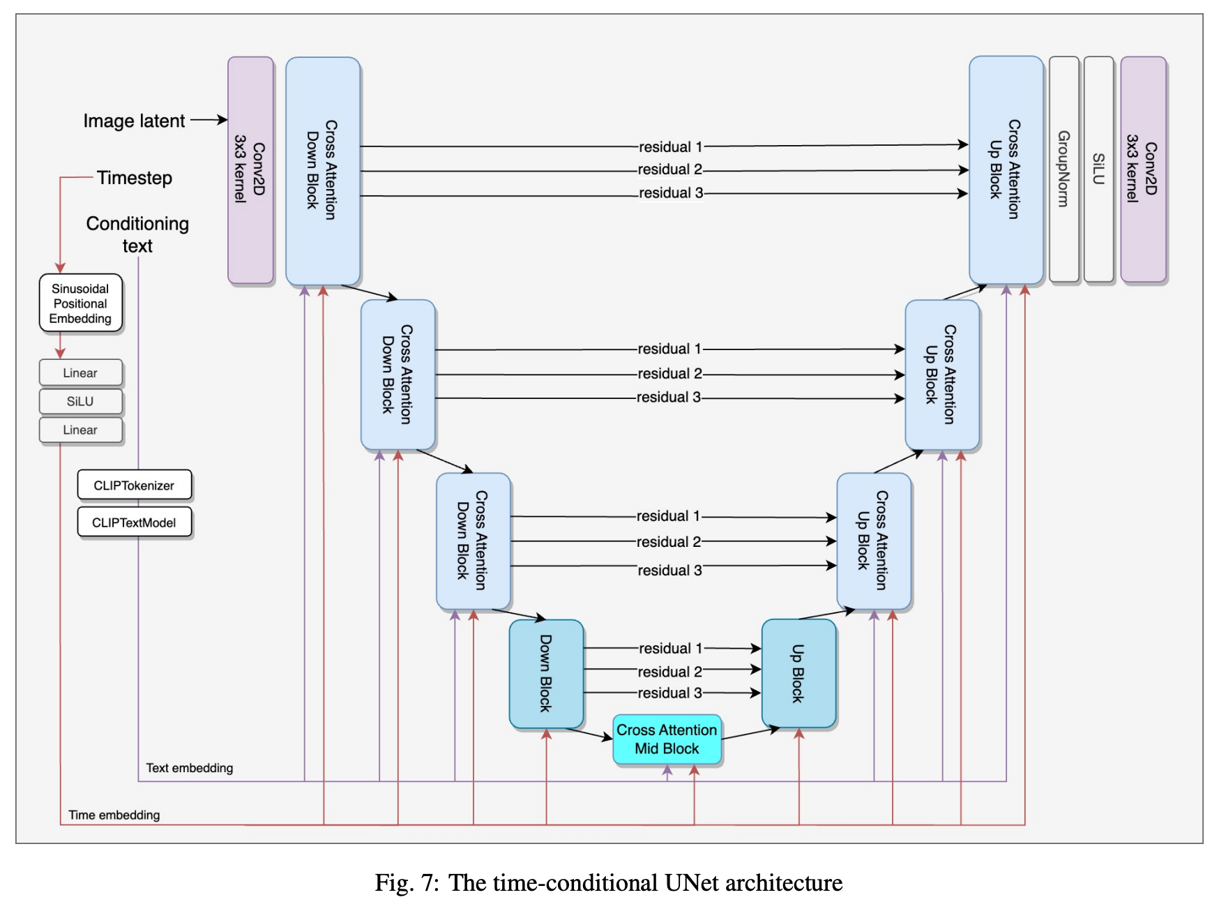
Note: this structure is based on version SD2.1, and the conditioning used is text conditioning. Compared with SD1.5, the main change is that the text encoder is replaced from CLIP ViT-L/14 with OpenCLIP-ViT/H; the rest is basically the same.
From the figure above we can see that, compared with the original UNet, the main change is that the original convolution structures are replaced by the Cross Attention Down Block, Down Block, Cross Attention Mid Block, Up Block and Cross Attention Up Block modules, and that time embedding and condition embedding (text embedding in the figure) are added as extra inputs.
Extra inputs
First the time embedding. According to the forward process of diffusion models, we have a timestep, and the goal of the UNet is to predict the random noise added at each timestep during the forward process, so the timestep is necessary information for the UNet. Following the transformer approach, sinusoidal positional embedding is applied to the timestep, and then two linear layers give the time embedding.
The condition embedding requires a different network to extract features depending on the type of conditioning. For example, the figure shows the text type, for which the corresponding model used is OpenCLIP.
Extra modules
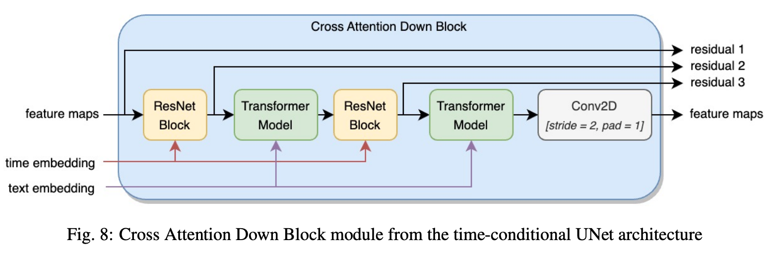
As for the Cross Attention Down Block and Cross Attention Up Block modules, the structure of the Cross Attention Down Block is as follows:
The structure of the Cross Attention Up Block is as follows:
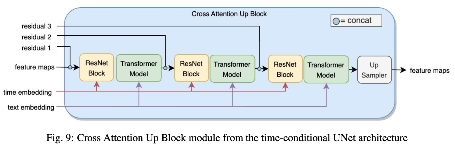
In both modules above, the time embedding only interacts with the ResNet Block, while the condition embedding participates in the Transformer Model through cross attention.
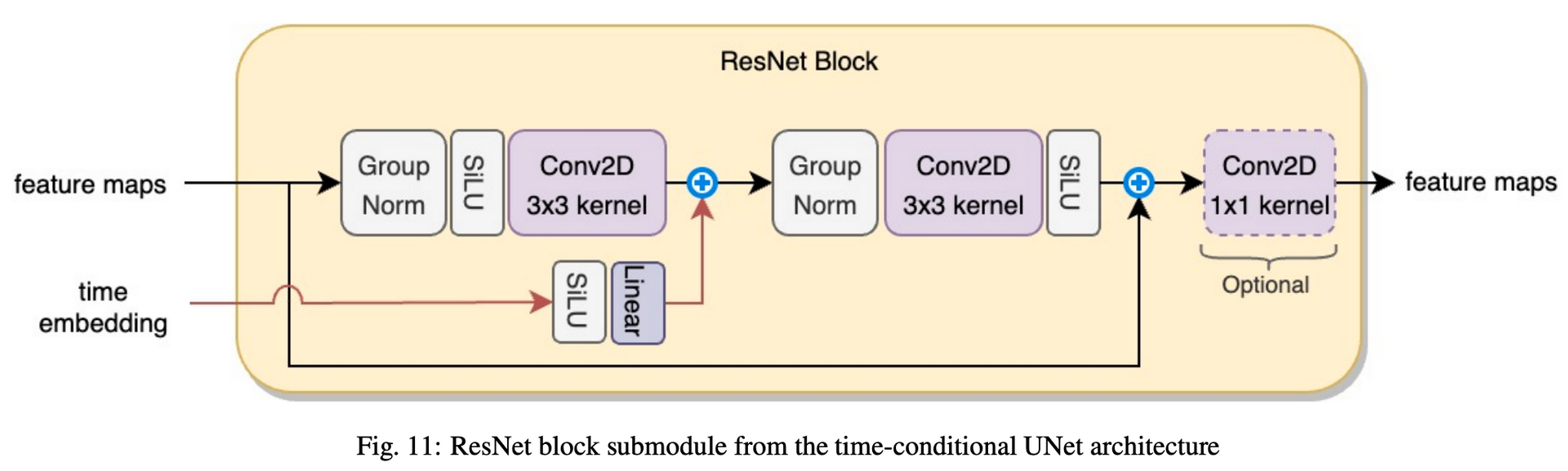
The detailed structure of the ResNet Block is as follows. The time embedding is mapped by a linear layer to a suitable size so that it can be added element-wise to the output of the convolution layer. The final $1\times 1$ convolution is optional and is meant to adjust the number of channels of the output feature map.
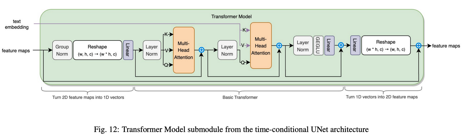
The detailed structure of the Transformer Model is as follows. This structure can be divided into three parts. The first part converts the input feature map into one-dimensional vectors and outputs them to the transformer. The second part is a regular transformer, in which the K and V values of the second Multi-Head Attention are produced by the condition embedding. The third part converts the one-dimensional vectors output by the transformer back into a feature map of the same size as the input.
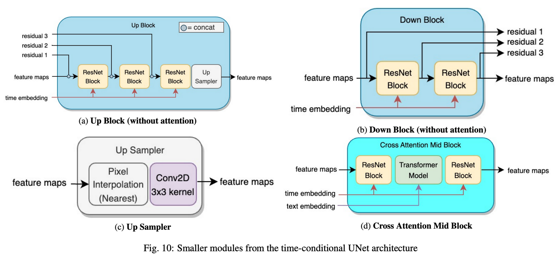
The structures of the remaining modules (Up Block, Down Block and Cross Attention Mid Block) are as follows:
Appendix
The differences between the latent diffusion model and the stable diffusion model (the two models are basically the same in structure):
- Compared with the training data of Latent diffusion (LAION-400M), stable diffusion was trained on a much larger amount of data (LAION-2B-en), and the data was also pre-filtered, so the quality is somewhat higher
- The text encoder used in the latent diffusion model is a randomly initialized transformer (that is, trained from scratch), whereas the stable diffusion model uses a pretrained CLIP model
- The training sizes are also different. For example, the latent diffusion model was only trained at a resolution of $256\times 256$, whereas the stable diffusion model is first pretrained at $256\times 256$ and then fine-tuned at $512\times 512$
For a more detailed answer, see here
The differences between the various versions of Stable diffusion. Since stable diffusion was released, the official team has put out many versions of the SD model, but the changes in principles and structure among these models are in fact not large; the differences are more likely in generation style.
- The text encoder of SD 1.x uses OpenAI’s CLIP ViT-L/14 model, with 123.65M parameters, whereas SD 2.0 uses a larger text encoder: the CLIP ViT-H/14 model trained on the laion-2b dataset based on OpenCLIP, with 354.03M parameters
- In the text encoder, SD 1.x extracts the features of the last layer. Since the features of the last layer are immediately followed by CLIP’s contrastive learning task, the last layer’s features may have partly lost fine-grained semantic information. SD 2.0 extracts the features of the second-to-last layer of the text encoder
- The attention modules at different stages in SD 2.0 fix the attention head dim to 64, whereas SD 1.x uses a fixed number of attention heads for the attention modules at different stages; clearly the SD 2.0 setting is more common, but this change does not affect the model parameters
- As for the training data, the SD 1.x version actually ended up mainly using the subset of LAION-2B with an aesthetic score of 5 or above, whereas the SD 2.0 version uses the subset with a score of 4.5 or above, which amounts to enlarging the training dataset
For more details, see here
Reference
High-Resolution Image Synthesis with Latent Diffusion Models
The Unreasonable Effectiveness of Deep Features as a Perceptual Metric
The Big Data Myth: Using Diffusion Models for Dataset Generation to Train Deep Detection Models
Latent Diffusion(Stable-Diffusion) Model (video)
Latent Diffusion(Stable-Diffusion) Model (pdf)
The Illustrated Stable Diffusion
A Beginner’s Guide to Variational Methods: Mean-Field Approximation